
Designing products with WGANs
This post elaborates on the idea of using Generative Adversarial Networks to design new products, such as car rims. Every time a company is looking for a new design of a product, hundreds of designers start their work and produce multiple suggestions each. Given the nature of the business, only one out of these suggestions is going to be implemented in the end, with the all other suggestions mostly thrown away. This large inefficiency could be resolved by the possibility of creating new design suggestions as easy as a click on a button. This is where GANs come in. By feeding them with images of already existing and economically successful images, the model is ultimately able to generate new design suggestions which are not possible to tell apart from real ones. For that purpose we used a few images car rims and implemented a Wasserstein GAN with Gradient Penalty in order to see how well the model can generate new design suggestions.
The post starts with a brief discussion about the history of GANs, before elaborating on the use case of design and fashion. Afterwards the data for this project is introduced and some data processing steps are introduced. Finally we show the Python code with which this project is implemented and conclude with the results in the end. For a more mathematical introduction to GANs and WGANs, please refer to my previous post about this topic.
GAN and WGAN
Since 2014 and the first paper of Generative Adversial Networks [1], it became difficult to keep track of all papers suggesting new implementation of GAN models. Arguably the most significant during the time right after the original papers was the addition of Deep Convolutional Neural Networks to GANs [2]. This method was particularly favorable for image data. As already outlined in my previous post, GANs are relatively instable and oftentimes get stuck during their training process. There are multiple potential reasons for a GAN model to get stuck, ranging from mode collapse over to vanishing gradients. One rather successful solution to this failures is the in 2017 proposed Wasserstein GAN (WGAN)[3].
The main difference between the Wasserstein GAN and “ordinary” is the way the model measures the distance between real data and generated fake data. Whereas the traditional GAN model is using the so-called Jenson-Shannon Divergence, the Wasserstein GAN is using, as the name already suggests the Wasserstein divergence. The main benefit of Wasserstein is that it does not diverge when the distributions of real and fake data are fairly far away from one another. Knowing how far away two distributions are from one another is crucial, since this information is used to update the weights of the Neural Network the generative model comprises of. These updates are conducted through Backpropagation and is the central mechanism of how the generative model improves over time. By telling the model how good or bad it created new fake data, the model has then the chance to use that feedback to improve in its next iteration. Therefore, it is detrimental if the measure of how bad the model is, is diverging. In this case, very bad and “normal” bad are quantitatively the same, and the model has a harder time to improve from these situations. Using the Wasserstein Distance is therefore to be preferred. For a more elaborated explanation of GANs and WGANs as well as a high level mathematical explanation of their foundations, please refer to my previous blog-post about the fundamental concept of GANs.
… and gradient penalty
Even though the Wasserstein paper rightfully claimed a lot of fame, it had one flaw. The way the Wasserstein paper is calculating the gradient update for the generative model is by using gradient clipping. That literally means that the gradients have to be in the range of -0.01 and 0.01. Everything bigger or smaller than this range is simply cut. As the paper states:
Weight clipping is a clearly terrible way to enforce a Lipschitz constraint… However, we do leave the topic of enforcing Lipschitz constraints in a neural network setting for further investigation, and we actively encourage interested researchers to improve on this method.
This call for improvement was also quickly heard. In the same year, Gulrajani et al published an improved version [4]. This new version of the Wasserstein GAN is using some heavy mathematics (check the appendix of the original paper if you feel like it) to implement a gradient penalty which does not require any unfavorable weight clipping anymore.
GANs and its applications in Design and Fashion
The range of use cases for GANs are immense. Furthermore, next to many flashy applications, GANs can also help to mitigate several real-life problems. One of which is the workings of the creative industry. Design and fashion are fields in which an insane amount of manual labor is constantly thrown away. In this day and age, the design of products became at least as important as its functionality. Whenever a company is planning to launch a new product, hundreds of designers submit multiple design suggestions, hoping to please the lead-designer. Since there is mostly one product and one design, all design suggestion except for one are being left unused and forgotten. The amount of inefficiency is arguably as large as the frustration of many designers, working long hours for nothing.
The described scenario would be different if new design suggestions would come as easy as a click on a button. This is where the GAN comes in. Being able to take inspiration by many other products, a GAN model could come up with a design which looks different but indistinguishable to the design of an already existing (and potentially approved) designs.
Use Case: Car Rim Design
To showcase the power of Generative Adversial Networks within the field of design, we chose to create new designs for car rims. Car rims have the benefit that they mostly are not overly complicated in regards to their design. This comes beneficial since generating a new image out of nothing but thin air is quite a difficult task even for neural networks.
Since the GAN is expected to learn which design patterns are acceptable for car rims, it is important to provide the model with a good quality of images. That means that there should be minimal noise, meaning no distraction factors. The best case scenario would therefore be if the images are all shoot from the same angle and also cropped similarly. Furthermore, having gray-scale images also helps since the model then has to learn only a third of the pixel values.
Trying to satisfy the outlined criteria above is difficult, since when blindly looking for new images, one rarely finds a whole lot of images shoot in a very similar way. Oftentimes we find a car attached to the rims (surprise), and other distortions like angle and cropping.
For that reason we looked at the different rim dealerships, as they sometimes provide all their products lined up in a very similar fashion. Our search led us to imagewheels.co.uk, which provided images of car rims in a favorable way. Not only did they shoot every photo nearly exactly the same, they also provided a dark background. This is beneficial to the model given that the GAN can therefore solely focus on the rim instead of the noise going on in the background.
import os
import numpy as np
from PIL import Image
import matplotlib.pyplot as plt

number_of_examples = 5
original_filenames = os.listdir("../data/original")[:number_of_examples]

fig, axs = plt.subplots(figsize=(20, 10), ncols=len(original_filenames))
for i, file_name in enumerate(original_filenames):
    image = Image.open(f"../data/original/{file_name}")
    np_array = np.array(image)
    axs[i].imshow(np_array)
    axs[i].axis("off")
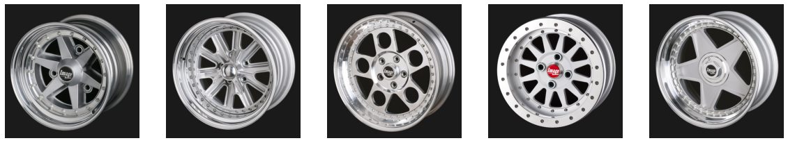
The images above show some examples of the images taken from the website. Even though the images are mostly gray, they still have three color channels, and therefore significantly more pixel values than gray-scale images. Since we are only interested in the overall design of the rim and not at all in its coloring, we therefore convert the image to gray-scale. Additional to that, we are reducing the complexity of the images even further, by turning every pixel value of the image either into black or white.
Even though the background of the sample images above looks entirely black, their pixel value is not exactly completely black. Therefore we manually help a bit. We do that by first checking which pixel value the very top left corner is. This pixel value then serves us as an indicator of what the background pixel value is, through which we can subset the image and turn everything (truly) black.
Additionally we only want to put emphasis on brighter details. That means that we paint everything black that is below a certain threshold level. That threshold is subjective and was manually adjusted until a sweet spot was found which left enough details of the rims. The resulting image can be seen below.
background_color = 255
detail_color = 0
threshold_level = 50

fig, axs = plt.subplots(figsize=(20, 10), ncols=len(original_filenames))
for i, file_name in enumerate(original_filenames):
    image = Image.open(f"../data/original/{file_name}")
    np_array = np.array(image)

    # Adjustments
    current_background_color = np_array[0][0]
    np_array[np_array==current_background_color] = background_color

    np_array[np_array<threshold_level] = background_color
    np_array[np_array!=background_color] = detail_color

    axs[i].imshow(np_array, cmap="gray")
    axs[i].axis("off")
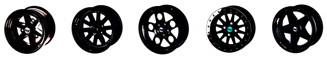
From the examples above one can clearly see the difference before and after our adjustment. Turning the car rims into black and white created a better contrast, and it became easier to identify the overall design.
The major drawback of our data is the limited amount we are working with. Even though the images are all nicely standardized, since they come from the same website, the price for that is that we can only take as many images as there are shown on the website. That left us with around 100 images, which is not a lot when working with GANs. Nevertheless, the GAN was able to produce some decent rim designs as we will see in the end of this post.
Code Implementation
As already mentioned in the beginning of this post, we are using a Wasserstein GAN with gradient penalty. The difference to a basic DCGAN is though only visible in the implementation of the Discriminator, which because of the adjustments is now called the critic. The main difference is that the output of the critic is not a probability of the image being real, which is the case for the generator. Furthermore, the usage of the Wasserstein divergence instead of the Jenson-Shannon divergence prevents most mode collapses and the vanishing of gradients. A more technical explanation of these phenomena can be found in my previous post.
In contrast to many GAN implementations on the web, I packaged my code which allows for easier changing of parameters and usage through the terminal. To give a good overview how the different files interact, we take a look into the folder structure.
import seedir as sd
sd.seedir("../source", style="lines", exclude_folders="__pycache__")
source/
├─.DS_Store
├─config.json
├─utils/
│ ├─config.py
│ └─args.py
├─generator.py
├─loader.py
├─trainer.py
├─critic.py
└─main.py
Loader
The first thing we have to do on our GAN model is to prepare the images. For that we apply the adjustment we outlined above and turn the colored images into black and whites. Furthermore, we resize them. This is necessary since the original images are quite large. When working with GANs, one has to be aware that the bigger the desired output image is, the more training is required. For that reason, most GANs are using no images bigger than 128x128 (with some exceptions of course). In our case we are working with even smaller images, namely 64x64. The benefit of using the smaller images size is that the model is able to mimic the distribution of real images faster. Though, smaller images also contain a lower level of detail, therefore it is a bit of a trade-off.
Furthermore, we normalize the image in order for them to have a mean and standard deviation equal to 0.5 each. This normalization of input values is necessary in order to stabilize the model and is done not only for GANs, but for every neural network application.
### loader.py

# %% Packages

import os
from PIL import Image
import numpy as np
import matplotlib.pyplot as plt
import torch
import torchvision.transforms as transforms
import torchvision.datasets as dset
import torchvision.utils as vutils

# %% Class


class DataLoader:

    def __init__(self, config):
        self.config = config
        self.base_dir = os.getcwd()

        self.create_black_white_images()
        self.loader = self.load_images()

    def load_images(self):
        """
        Loading the black and white images and transforming them accordingly
        :return: Returning a dataloader from PyTorch
        """
        transform = transforms.Compose([
            transforms.Grayscale(),
            transforms.ToTensor(),
            transforms.Normalize(0.5, 0.5)
        ])

        dataset_path = f"{self.base_dir}/data/black_white"
        dataset = dset.ImageFolder(root=dataset_path, transform=transform)
        loader = torch.utils.data.DataLoader(dataset, batch_size=self.config.loader.batch_size, shuffle=True)
        self.plot_example_images(loader)

        return loader

    def plot_example_images(self, loader):
        """
        Using the data loader in order to plot some example images
        :param loader: DataLoader from PyTorch
        """
        example_images, _ = next(iter(loader))[:self.config.loader.batch_size]
        fig, axs = plt.subplots(figsize=(20, 10))
        axs.axis("off")
        axs.set_title("Example Images")
        batch_images = vutils.make_grid(example_images, padding=True, normalize=True)
        image_grid = np.transpose(batch_images, (1, 2, 0))
        axs.imshow(image_grid)
        fname = f"{self.base_dir}/reports/figures/example_images.png"
        fig.savefig(fname=fname, bbox_inches="tight")
        plt.close()

    def create_black_white_images(self):
        """
        Creating the black and white versions of the original images
        """
        if self.config.loader.create_new_images:

            all_file_names = os.listdir("./data/original")

            for i, file_name in enumerate(all_file_names):
                image = Image.open(f"{self.base_dir}/data/original/{file_name}").convert("L")
                resized_image = image.resize(
                    (self.config.loader.target_size, self.config.loader.target_size)
                )

                np_array = np.array(resized_image)

                current_background_color = np_array[0, 0]
                np_array[np_array==current_background_color] = self.config.loader.background_color

                np_array[np_array<self.config.loader.detail_color_level] = self.config.loader.background_color
                np_array[np_array!=self.config.loader.background_color] = self.config.loader.detail_color_level

                im = Image.fromarray(np_array)
                saving_path = f"{self.base_dir}/data/black_white/images/{i}.jpg"
                im.save(saving_path)
Generator
The generator of this GAN model is exactly the same as for a DCGAN. That is because all adjustments of the Wasserstein divergence and gradient penalty are made on the discriminator (which is therefore called the critic instead).
In contrast to other implementations online, we are using LeakyRelU instead “normal” RelU. That is because of the suggestions of ganhacks. According to this guideline, which is written by Facebook AI research, it is also advised to use a dropout layer at multiple layers of the generative model, which we therefore also do. Though instead of using a dropout level of 0.5, as the guide suggests, we are using only 0.2, since the lower rate proved to result in better images in our scenario.
From the in-line comments of the code below we can nicely see how the size of the image increases over time. Starting with an image size of 4x4, we slowly work our way up, until we get to the desired image size of 64x64. When implementing any convolution model, it is always worthwhile to do the arithmetic, in order to see whether the specifications for padding, stride and etc. work out. We have to be a bit careful in this scenario, as we are using convolution transpose to increase the image size. The formula of how to calculate the resulting image size given the input parameters is stated below. Note that since we are working with square images, we are only showing the calculation for the height of the image, which is denoted by $H$. Additionally, the stride is denoted as $S$, the padding as $P$, the dilation as $D$ and the kernel size as $K$.
\[\begin{align} H_{out} = \left( H_{in} - 1 \right) \cdot S - 2 \cdot P + D \cdot \left( K - 1 \right) + 1 \end{align}\]Applying the formula above on our data, we then can calculate the size of the image at every layer. The following table summarizes the results of these calculations. Note that for the first layer we did not state an input size as here the noise vector is simply projected to the size of the kernel.
| Layer Number | Input Size | Kernel Size | Stride | Padding | Dilation | Output Size |
|---|---|---|---|---|---|---|
| 1 | / | 4 | 1 | 0 | 1 | 4 |
| 2 | 4 | 4 | 2 | 1 | 1 | 8 |
| 3 | 8 | 4 | 2 | 1 | 1 | 16 |
| 4 | 16 | 4 | 2 | 1 | 1 | 32 |
| 5 | 32 | 4 | 2 | 1 | 1 | 64 |
### generator.py

# %% Packages

import torch.nn as nn

# %% Class


class Generator(nn.Module):

    def __init__(self, config):
        self.config = config
        super(Generator, self).__init__()
        fm = self.config.model.feature_maps

        self.main = nn.Sequential(
            self._block(self.config.model.noise_dim, fm * 16, kernel_size=(4, 4), stride=(1, 1), padding=(0, 0)),  # 4
            self._block(fm * 16, fm * 8, kernel_size=(4, 4), stride=(2, 2), padding=(1, 1)),  # 8
            self._block(fm * 8, fm * 4, kernel_size=(4, 4), stride=(2, 2), padding=(1, 1)),  # 16
            self._block(fm * 4, fm * 2, kernel_size=(4, 4), stride=(2, 2), padding=(1, 1)),  # 32
            nn.ConvTranspose2d(fm * 2, 1, kernel_size=(4, 4), stride=(2, 2), padding=(1, 1)),  # 64
            nn.Tanh()  # [-1, 1]
        )

    def _block(self, in_channels, out_channels, kernel_size, stride, padding):
        return nn.Sequential(
            nn.ConvTranspose2d(in_channels, out_channels, kernel_size, stride, padding),
            nn.BatchNorm2d(out_channels),
            nn.LeakyReLU(self.config.model.leaky_relu_rate, inplace=True),
            nn.Dropout(self.config.model.dropout_rate)
        )

    def forward(self, input):
        output = self.main(input)
        return output
Critic
The main difference between the critic and the discriminator is that the output of this model is not normalized between 0 and 1 anymore. Instead of providing probabilities how certain the model is that the image is real, the critic is simply outputting the value of its loss function. This method has the benefit of making the generator understand better how far away the fake data distribution is from the distribution of the real images.
In contrast to the generator, the critic is using traditional convolutions. Therefore, the formula to calculate the outputted image size given certain input parameters is a bit different. Using the same notation for padding, stride and etc., the formula is:
\[\begin{align} H_{out} = \frac{H_{in} + 2 \cdot P - D \cdot \left( K - 1 \right) - 1}{S} + 1 \end{align}\]Following that formula the we quickly also find how the image size is reduced from 64x64 down to one number, meaning a size of 1x1.
| Layer Number | Input Size | Kernel Size | Stride | Padding | Dilation | Output Size |
|---|---|---|---|---|---|---|
| 1 | 64 | 4 | 2 | 1 | 1 | 32 |
| 2 | 32 | 4 | 2 | 1 | 1 | 16 |
| 3 | 16 | 4 | 2 | 1 | 1 | 8 |
| 4 | 8 | 4 | 2 | 1 | 1 | 4 |
| 5 | 4 | 4 | 2 | 0 | 1 | 0 |
### critic.py

# %% Packages

import torch.nn as nn

# %% Class


class Critic(nn.Module):
    def __init__(self, config):
        self.config = config
        super(Critic, self).__init__()
        fm = self.config.model.feature_maps

        self.main = nn.Sequential(  # 64
            nn.Conv2d(1, fm * 2, kernel_size=(4, 4), stride=(2, 2), padding=(1, 1)),  # 32
            nn.LeakyReLU(0.2, inplace=True),
            self._block(fm * 2, fm * 4, kernel_size=(4, 4), stride=(2, 2), padding=(1, 1)),  # 16
            self._block(fm * 4, fm * 8, kernel_size=(4, 4), stride=(2, 2), padding=(1, 1)),  # 8
            self._block(fm * 8, fm * 16, kernel_size=(4, 4), stride=(2, 2), padding=(1, 1)),  # 4
            nn.Conv2d(fm * 16, 1, kernel_size=(4, 4), stride=(2, 2), padding=(0, 0), bias=False),  # 1
        )

    def _block(self, in_channels, out_channels, kernel_size, stride, padding):
        return nn.Sequential(
            nn.Conv2d(in_channels, out_channels, kernel_size, stride, padding, bias=False),
            nn.InstanceNorm2d(out_channels),
            nn.LeakyReLU(self.config.model.leaky_relu_rate, inplace=True)
        )

    def forward(self, input):
        output = self.main(input)
        return output
Trainer
The models are then loaded into the training class. The training class starts by initializing the weights of the generator and the critic, before setting up the optimizers. Following the suggestions from ganhacks, we are using the Adam optimizer. The learning rate, as well as the values for the betas are taken from the original paper, namely 1e-4.
Note that we are creating some “constant” noise which is used to see how our generative model improves over time. Through the constant noise we can plot the output of the very same input after every adjustment of the model in order to see the change in output. The emphasis on visualization at various points is also one of the main reasons why this class contains so many more lines of code compared to the other files. Given that GANs do not have a objectively agreed on loss function to assess model performance, the visual inspection of results is particularly important.
Given that we are working with a relatively small amount of images (around 100), we have to ramp up the number of epochs the model is training with. In contrast to 50 epochs, which is used for example in the tensorflow guide when generating new MNIST pictures, we are using 1000 epochs. The small amount of images also reduces the batch size we can use. In contrast to the usual 32, 64, or even 128, we are using a batch size of a mere 8.
### trainer.py

# %% Packages

import os
import datetime
import matplotlib.pyplot as plt
import numpy as np
import imageio
import torch
import torchvision
import torch.nn as nn
import torch.optim as optim
from torch.utils.tensorboard import SummaryWriter

# %% Class


class GanTrainer:

    def __init__(self, generator, critic, data, config):
        self.generator = generator
        self.critic = critic
        self.data = data
        self.config = config
        self.device = "cpu"

        # Initialization empty containers
        self.generator_loss = []
        self.critic_loss = []
        self.image_list = []

        # Creation of tensorboard and training model
        self.sw_real, self.sw_fake = self.create_tensorboard()
        self.train_gan()

    def gradient_penalty(self, critic, real, fake):
        """
        This method calculates the gradient penalty, which is the essential component of the WGAN with
        gradient penalty
        :param critic: Critic Model
        :param real: Batch of real images
        :param fake: Batch of fake images created by the generator
        :return:
        """
        batch_size, c, h, w = real.shape
        epsilon = torch.rand((batch_size, 1, 1, 1)).repeat(1, c, h, w).to(self.device)
        interpolated_images = real * epsilon + fake * (1 - epsilon)

        mixed_scores = critic(interpolated_images)
        gradient = torch.autograd.grad(
            inputs=interpolated_images,
            outputs=mixed_scores,
            grad_outputs=torch.ones_like(mixed_scores),
            create_graph=True,
            retain_graph=True
        )[0]

        gradient = gradient.view(gradient.shape[0], -1)
        gradient_norm = gradient.norm(2, dim=1)
        gradient_penalty = torch.mean((gradient_norm - 1) ** 2)

        return gradient_penalty

    def create_tensorboard(self):
        """
        Setting up the tensorboard
        :return:
        """
        sw_real = SummaryWriter(f"./logs/{datetime.datetime.now():%Y-%m-%d}/real")
        sw_fake = SummaryWriter(f"./logs/{datetime.datetime.now():%Y-%m-%d}/fake")
        return sw_real, sw_fake

    def weights_init(self, m):
        """
        Weight initialization method for the generator and critic
        :param m: The inputted model (either generator or critic)
        :return:
        """
        classname = m.__class__.__name__
        if classname.find("Conv") != -1:
            nn.init.normal_(m.weight.data, 0.0, 0.02)
        elif classname.find("BatchNorm") != -1:
            nn.init.normal_(m.weight.data, 1.0, 0.02)
            nn.init.constant_(m.bias.data, 0)

    def plot_losses(self):
        """
        Method to plot the loss function of critic and generator
        :return:
        """
        fig, axs = plt.subplots(figsize=(20, 5))
        axs.plot(self.generator_loss, label="Generator Loss")
        axs.plot(self.critic_loss, label="Critic Loss")
        axs.set_xlabel("Iterations")
        axs.set_ylabel("Loss")
        axs.legend()
        fname = "./reports/figures/loss.png"
        fig.savefig(fname=fname, bbox_inches="tight")
        plt.close()

    def save_epoch_image(self, grid, epoch):
        """
        Saving a snapshot of fixed noise in order to see the progress made by the mode
        :param grid: Grid from PyTorch
        :param epoch: Integer indicating which epoch we are at
        :return:
        """
        fig, axs = plt.subplots(figsize=(10, 10))
        image_grid = np.transpose(grid, (1, 2, 0))
        axs.imshow(image_grid)
        axs.axis("off")
        axs.set_title(f"Fake Images at Epoch Number {epoch}")

        fname = f"./reports/epoch_examples/epoch_{epoch}.png"
        fig.savefig(fname=fname, bbox_inches="tight")
        plt.close()

    def save_model(self):
        """
        Saving the generator model in order to be used outside of the trainer.py
        :return:
        """
        model_path = "./model/generator.h5"
        torch.save(self.generator.state_dict(), model_path)

    def build_gif(self):
        """
        Method which builds a gif from all the snapshots created. This helps assess progress made by the model
        :return:
        """
        images = []
        file_names = os.listdir("./reports/epoch_examples")
        file_names.sort(key=lambda x: float(x.strip("epoch_").strip(".png")))
        for file in file_names:
            images.append(imageio.imread(f"./reports/epoch_examples/{file}"))
        imageio.mimsave("./reports/figures/epoch.gif", images)

    def train_gan(self):
        """
        Training the model in its entirety
        :return:
        """
        self.generator.apply(self.weights_init)
        self.critic.apply(self.weights_init)

        optimizer_generator = optim.Adam(
            self.generator.parameters(), lr=self.config.trainer.learning_rate, betas=(0.0, 0.9)
        )
        optimizer_critc = optim.Adam(
            self.critic.parameters(), lr=self.config.trainer.learning_rate, betas=(0.0, 0.9)
        )

        constant_noise = torch.randn(
            self.config.trainer.number_of_examples, self.config.trainer.noise_dimension, 1, 1, device=self.device
        )

        self.generator.train()
        self.critic.train()

        global_step = 0
        for epoch in range(self.config.trainer.number_of_epochs):

            for real_image, _ in self.data.loader:
                current_batch_size = real_image.shape[0]

                # Critic Training
                for _ in range(self.config.trainer.critic_iterations):

                    noise = torch.randn(
                        current_batch_size, self.config.trainer.noise_dimension, 1, 1, device=self.device
                    )
                    fake_image = self.generator(noise)
                    critic_real = self.critic(real_image).reshape(-1)
                    critic_fake = self.critic(fake_image).reshape(-1)
                    gradient_penalty = self.gradient_penalty(self.critic, real_image, fake_image)
                    loss_critic = (
                        - (torch.mean(critic_real) - torch.mean(critic_fake))
                        + (self.config.trainer.lambda_gp * gradient_penalty)
                    )
                    self.critic.zero_grad()
                    loss_critic.backward(retain_graph=True)
                    optimizer_critc.step()

                # Generator Training
                gen_fake = self.critic(fake_image).reshape(-1)
                loss_gen = -torch.mean(gen_fake)
                self.generator.zero_grad()
                loss_gen.backward()
                optimizer_generator.step()

            # Print losses occasionally and print to tensorboard
            if epoch % self.config.trainer.print_epochs_after == 0 and epoch > 0:
                print(
                    f"Epoch [{epoch}/{self.config.trainer.number_of_epochs}] "
                    f"Loss D: {loss_critic:.4f}, loss G: {loss_gen:.4f}"
                )
                self.plot_losses()
                self.save_model()
                self.build_gif()

            # Tensorboard
            with torch.no_grad():
                fake_examples = self.generator(constant_noise)
                real_examples = real_image[:self.config.trainer.number_of_examples]

                img_grid_real = torchvision.utils.make_grid(real_examples, padding=1, normalize=True)
                img_grid_fake = torchvision.utils.make_grid(fake_examples, padding=1, normalize=True)

                self.sw_real.add_image("Real", img_grid_real, global_step=global_step)
                self.sw_fake.add_image("Fake", img_grid_fake, global_step=global_step)

                # Filling containers
                self.generator_loss.append(loss_gen.item())
                self.critic_loss.append(loss_critic.item())

                # Save epoch example image
                self.save_epoch_image(img_grid_fake, epoch)

                global_step += 1
Main
Lastly we import all priorly shown files into the main.py and execute the code from the terminal. It is to be said that GANs take a very long time to train, especially when one’s computer does not have a GPU. In order to speed up training, one could either use a cloud solution, or make use of Google Colab’s free (but limited) usage.
One of the main benefits of the usage of a config file, like we do, is that the user can easily change several parameters of the model, without having to step into any of the Python scripts. This is especially convenient for users external to the development of this project.
### main.py

# %% Packages

from utils.args import get_args
from utils.config import process_config
from loader import DataLoader
from critic import Critic
from generator import Generator
from trainer import GanTrainer

# %% Script


def main():

    args = get_args()
    config = process_config(args.config)

    print("Load Discriminator")
    critic = Critic(config)

    print("Load Generator")
    generator = Generator(config)

    print("Load Data")
    data = DataLoader(config)

    print("Training the model")
    trainer = GanTrainer(generator, critic, data, config)


if __name__ == "__main__":
    main()
Results
After training the model for around a day, we find some decent results. Below one can see the progress the model made from the very beginning. It is nicely visible that the model started with a black blob, but then quickly started to recognize the need for a round shape and some white spots in the middle. It then took the model quite a bit more time before recognizing what kind of design the rims are supposed to have in order to be mistaken for a real one. After around 300-400 epochs there is not too much change anymore and the model performance stagnates. At this point one could have already stopped training as not much is happening more. One way to get a higher level of detail would be to increase the image size, since details would then be easier to spot for the model.
One significant drawback of GANs is the lack of a proper loss function. Since the generator and the critic are playing against each other in some sort of a zero-sum game, it is unclear what kind of loss metric we should look at in order to assess the model performance. The usage of the Wasserstein divergence helps a bit here. That is because the original paper is documenting a correlation between the loss of the generative model and the overall image quality. However, the same paper also states that:
…we do not claim that this is a new method to quantitatively evaluate generative models yet. The constant scaling factor that depends on the critic’s architecture means it’s hard to compare models with different critics.
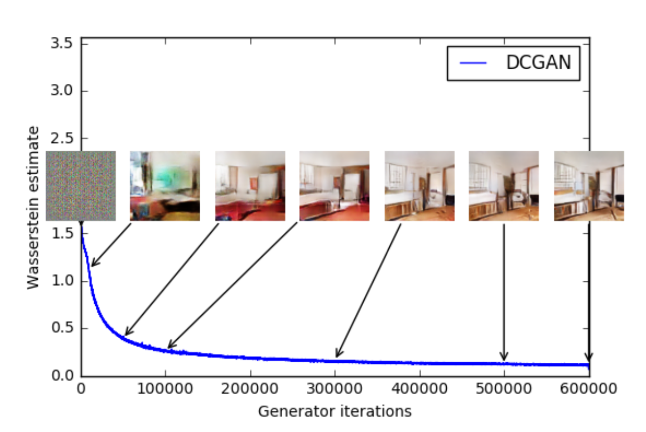
Contrasting that image from the original paper to our loss function, we can see from the blue line that an overall decline is visible. Therefore using the loss of the generative model could indeed serve us as an indication of how well the model is doing.
Outlook
Lastly, it to be said that we are overall quite happy with the results of our rim designs. In the future different implementations of GANs (e.g. StyleGans) could be tried in order to see whether a more satisfying results are obtainable. Additionally it would be beneficial to find a use-case for which we have more images. Especially the big design studios around the world must have tons of such data and it will be only a matter of time until your next T-Shirt is going to be designed by an AI.
Appendix
References
[1] - Goodfellow, Ian J., et al. “Generative adversarial networks.” arXiv preprint arXiv:1406.2661 (2014). APA
[2] - Radford, Alec, Luke Metz, and Soumith Chintala. “Unsupervised representation learning with deep convolutional generative adversarial networks.” arXiv preprint arXiv:1511.06434 (2015). APA
[3] - Arjovsky, Martin, Soumith Chintala, and Léon Bottou. “Wasserstein generative adversarial networks.” International conference on machine learning. PMLR, 2017.
[4] - Gulrajani, Ishaan, et al. “Improved training of wasserstein gans.” arXiv preprint arXiv:1704.00028 (2017).
Config File
import json

with open("../source/config.json") as json_file:
    config_file = json.load(json_file)
for key, value in config_file.items():
    print(key)
    print(value)
loader
{'create_new_images': False, 'target_size': 64, 'detail_color_level': 50, 'background_color': 255, 'detail_color': 0, 'batch_size': 8}
model
{'leaky_relu_rate': 0.2, 'noise_dim': 100, 'dropout_rate': 0.2, 'feature_maps': 64}
trainer
{'learning_rate': 0.0001, 'batch_size': 8, 'noise_dimension': 100, 'number_of_epochs': 1000, 'lambda_gp': 10, 'number_of_examples': 16, 'critic_iterations': 5, 'print_epochs_after': 5}