Dynamic Time Warping: Explanation and extensive testing on audio and tabular data

Explaining the concept of Dynamic-Time-Warping and testing it extensively on sound and tabular data.

Introduction

When working with time-series data, the question will at some point occur how to do time-series clustering. This question could occur in multiple scenarios and areas of Data Science.

For once it could happen when working with sound data. One could potentially try to cluster certain sound-waves together since they represent the same spoken word. Sound is a particularly interesting case, since we would also like the clustering algorithm to be invariant to time, since the same word could be spoken in different speeds. The machine should understand that when somebody says Hello or Heeeelllooo, they mean the same thing.

Another use case of time-series classification/ clustering is when trying to find which time-series are sufficiently similar in order to use them to build a pooled forecasting model. A pooled model describes situation in which we are not building one model for each time-series we would like to predict, but fitting one model on multiple entities. When doing that, we should be convinced that there is cross-learning potential. Therefore, trying to first cluster similar time-series together could substantial help to know which time-series could be jointly used for a pooled model.

Lastly, when working with time-series data, it could happen that two or more series have different lengths. This problem is oftentimes a deal-breaker for many models, as most classification/ cluster algorithms are not equipped to deal with a varying amount of features.

All of these problems can be solved with Dynamic Time Warping (DTW), which is the topic of this post. We start by showing a basic situation in which using the euclidean distance would lead us to the incorrect conclusion and show how DTW can be beneficial. Afterwards we elaborate on the mathematical idea of DTW and illustrate its workings, using a simple example. After that we implement the algorithm into Python code. In order to show the potential of DTW, we show-case different usage areas, ranging from sound-data of different complexity to tabular data.

We start the post by importing all the relevant packages we need later on. Note that we also import a self-written _config file in which only basic matplotlib settings are specified. Through importing these configurations in the beginning, we do not have to specify things like font-size every time we create a plot.

import os
import sys
import numpy as np
import pandas as pd
from tqdm import tqdm
from pydub import AudioSegment
import IPython.display as ipd

import matplotlib.pyplot as plt
from matplotlib.pyplot import cm
import seaborn as sns

from fastdtw import fastdtw
from tslearn.neighbors import KNeighborsTimeSeriesClassifier
from sklearn.model_selection import train_test_split
from sklearn.metrics import accuracy_score, f1_score, precision_score, recall_score
from scipy.spatial.distance import euclidean
from sklearn.ensemble import GradientBoostingClassifier
from sklearn.model_selection import GridSearchCV

sys.path.append("../src/")
import _config

DATA_PATH = "../data"
FIGURES_PATH = "../reports/figures"

Problem at hand

Given that the similarity between two time-series could be easily interpreted as the distance of two vectors, the idea could quickly arise to use the euclidean distance. The euclidean is defined as the sum of the squared elements of each corresponding element of two vectors. Or even more formal: The euclidean distance between vector p and q is defined as \(d(p, q) = \sqrt{\sum^n_{i=1} (q_i - p_i)^2}\).

As already visible by the subscript i for each element of p and q, it is necessary for both time series to have equal length. This of course is especially problematic with sound-data. Here it could happen that you say the same word at a different pace, which would lead the sound-files to have different lengths. One solution to that problem would be to simply clip the longer file, in order to match the size of the shorter file.

Below we find two functions for calculating the euclidean distance. The first implements the aforementioned clipping, whereas the second functions implements the calculation of the Euclidean distance.

def cut_time_series(array1, array2):
    length_array1 = len(array1)
    length_array2 = len(array2)
    if length_array1 < length_array2: # we have to clip the second series
        array2 = array2[:length_array1]
    else: # we have to clip the first series
        array1 = array1[:length_array2]
    return array1, array2

def euclidean_distance_calculator(array1, array2):
    clipped_array1, clipped_array2 = cut_time_series(array1, array2)
    assert len(clipped_array1) == len(clipped_array2), "Not equal length!"
    dist = np.linalg.norm(clipped_array1-clipped_array2)
    return round(dist, 2)

Even though the euclidean distance is a quickly understood and easily implementable method, it is heavily flawed when trying to find true similarities between different time-series. This is visualized through the example below. Here we have three Signals. The first two signals represent sine waves with a different frequency as well as amplitude. The third signal represents a mere straight line with a small slope.

AMPLITUDE1 = 1
AMPLITUDE2 = 3/4
SAMPLE_RATE = 8000
FREQUENCY1 = 6
FREQUENCY2 = 3
sample = 8000
time = np.arange(SAMPLE_RATE)
signal1 = AMPLITUDE1 * np.sin(2 * np.pi * FREQUENCY1 * time / SAMPLE_RATE)
signal2 = AMPLITUDE2 * np.sin(2 * np.pi * FREQUENCY2 * time / SAMPLE_RATE)
signal3 = (time * 0.00005) - 0.2

fig, axs = plt.subplots(figsize=(10, 10))
axs.plot(time, signal1, label="Signal 1")
axs.plot(time, signal2, label="Signal 2")
axs.plot(time, signal3, label="Signal 3")
axs.legend()
plt.show()

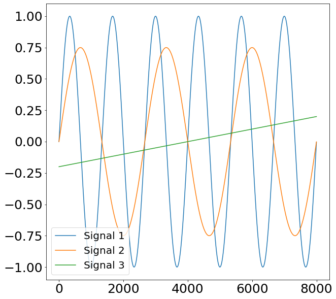
Given that the former two signals represent a sine curve, we would like our similarity algorithm to also find a bigger similarity (a.k.a smaller distance) between Signal 1 and 2 compared to Signal 3. When applying the euclidean distance to this problem we find the following:

print(f"The euclidean distance between Signal 1 and Signal 2 is {euclidean_distance_calculator(signal1, signal2)}")
print(f"The euclidean distance between Signal 2 and Signal 3 is {euclidean_distance_calculator(signal2, signal3)}")

The euclidean distance between Signal 1 and Signal 2 is 79.06
The euclidean distance between Signal 2 and Signal 3 is 51.1

As already feared, the euclidean distance suggests that Signal 2 and 3 are actually more similar than Signal 1. This behavior is, because of the aforementioned reasons, undesired. A powerful alternative of the euclidean distance is the so-called Dynamic-Time-Warping (DTW) distance. Using the fastdtw implementation, we find a result which aligns with our initial intuition.

print(f"The DTW distance between Signal 1 and Signal 2 is {round(fastdtw(signal1, signal2)[0], 2)}")
print(f"The DTW distance between Signal 2 and Signal 3 is {round(fastdtw(signal2, signal3)[0], 2)}")

The DTW distance between Signal 1 and Signal 2 is 2858.61
The DTW distance between Signal 2 and Signal 3 is 3993.83

The workings of Dynamic-Time-Warping

The fundamental differences between the euclidean distance and the DTW distance is that the former is simply comparing the sequences element by element, whereas the second algorithm is actively trying to look for the closest possible connections between two observations within each series.

To better show that, let us define the following two sequences: \(A = a[0], a[1], ..., a[n] \quad B = b[0], b[1], ..., b[m]\)

What DTW is now doing is that it tries to match element $a[i]$ to the closest element of B, regardless of whether it is also at position i. Hence it would be possible to connect element $a[i]$ with element $b[i+4]$, if that would minimize the distance between these two. This distance is oftentimes calculated by using the euclidean distance, but other distance measures are possible.

The magic of Dynamic-Time-Warping is the so-called Warping Path. The warping-path matches the different elements within A and B in such a way that the aggregated distance of all elements is minimized. Before showing how the warping function is doing that, we first introduce some boundaries on how the matching is allowed to happen.

Restrictions on Warping Function

As already mentioned, Dynamic-Time-Warping allows each element from one sequence to match with one or even multiple other elements from another series, even if this element is not at the same index position. Though, there are some restrictions on how DTW is allowed to do that. The original paper from Hiroaki Sakoe and Seibi Chiba 1978 [1] state the following five conditions.

1. Monotonic conditions This condition says that we are not allowed to match the following element, if we have not matched the current element already. Meaning that we are not allowed to go back in time \(i(k-1) \leq i(k) \quad \text{and} \quad j(k-1) \leq j(k)\)

2. Continuity conditions When finding the optimal warping path, we are not allowed to jump in time \(i(k) - i(k-1) \leq 1 \quad \text{and} \quad j(k) - j(k-1) \leq 1\)

3. Boundary conditions This condition ensures that both sequences start on their first element and end on their last element \(i(1) = 1, j(1) = 1 \quad \text{and} \quad i(K) = I, j(K) = J\)

4. Adjustment window condition This condition ensures that matching partners are not further apart than a predefined distance, defined by the positive integer r \(|i(k) - j(k)| \leq r\)

5. Slope constraint condition The slope constraint is put in place in order to prevent the warping path to go too extremely into one direction, which would lead to undesirable distortions

Distance Matrix

Now it is time to explore how the optimal warping path is found. In order to understand that, we have to introduce yet another concept, called the distance matrix. The concept of which is easily understood though. The distance matrix quantitatively describes the cost of each possible matching path between two or more sequences.

Building such a distance-matrix happens in two steps. The first step is to calculate some sort of a base-cost matrix. The second step is then to iteratively filling the distance-matrix, using the base-cost matrix from the first step. This base-cost describes the distance between every combination of points of two sequences. For illustrative purposes, consider the following two sequences:

array1 = [1, 2, 3, 4, 4, 4, 3, 2, 1]
array2 = [1, 3, 4, 4, 2, 1]

We then build a matrix which contains the distance between each combination of two elements from the sequences. As a measure for the distance we are using the squared distance between the two elements. The following function implements this for our two sequences. Note that we want the beginning of the two sequences to start in the lower left corner. In order for that to happen we have to reverse the second array.

def euclidean_distance_matrix(x, y):
    dist = np.zeros((len(y), len(x)))
    for i in range(len(y)):
        for j in range(len(x)):
            dist[i,j] = (x[j]-y[i])**2
    return dist
euc_array = euclidean_distance_matrix(array1, array2[::-1])
euc_df = pd.DataFrame(data=euc_array, columns=array1, index=array2)
fig, axs = plt.subplots(figsize=(20, 10))
sns.heatmap(euc_df, ax=axs, annot=True)
plt.show()

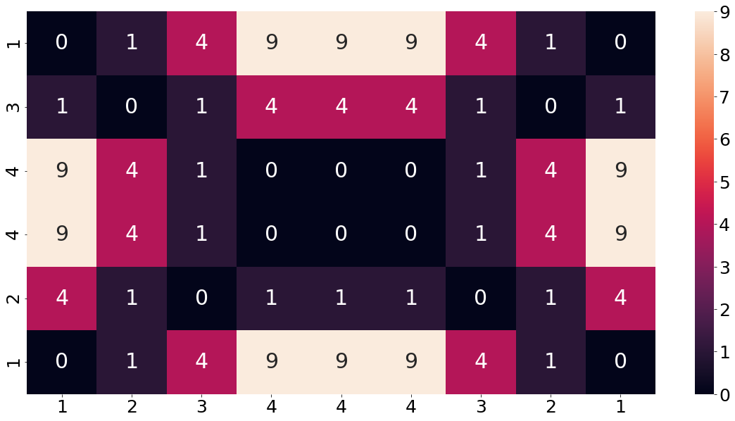
In order to make sure that the concept of the base-cost matrix is understood, let us consider an example from the chart above. For instance, the third cell from the top and second from the left. At this position the first array (shown on the columns) has a value of 2 and the second array (shown on the index) has a value of 4. The squared distance between these two elements is equal to 4, which is also shown in the matrix. This value of 4 can be understood as the cost of matching these two elements.

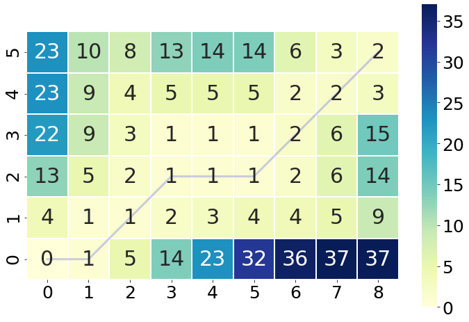
After we build the entire base-cost matrix, it is now time to fill the distance-matrix. Filling the distance-matrix does not happen all at once. Rather it happens one after another, since each element depends on the previously calculated value. This approach is also referred to as dynamic programming. A good analogy of understanding how we fill in the distance matrix is to imagine that we have a chess-king, which starts in the lower left of the matrix and then goes and explores every path of the matrix. For those who do not know, a chess king can only move one square at a time in every direction. The procedure begins by filling in the bottom left element of the base-cost matrix into our yet still empty distance matrix (in our case a zero).

The chess king then starts exploring the boundary cells of the distance-matrix. Every time the chess king moves to a new square he incurs the cost of the base-cost matrix, but he also drags with him the minimum adjacent cost of the squares behind him. The graphic below shows the result of that step. The calculation of the blue 22, for example was done by checking the base-cost element at that position (9) and summing the previous value to it (13). The same applies to the red 5 in the bottom row. Here again we first check the element of the base-cost matrix at that position (4) and sum the previous value (1) to it.

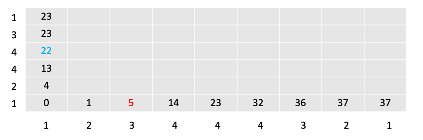
Again, at every step the chess king occurs the cost of the base-cost matrix at that position, plus the minimum value of the cells adjacently behind him: (i-1, j), (i, j-1) or (i-1, j-1). Or mathematically formulated: \(r(i, j) = d(x_i, y_j) + min\{r(i-1, j), \quad r(i, j-1), \quad r(i-1, j-1)\}\)

For which $d(x_i, y_j)$ describes the squared distance. Through this dynamic programming approach we then fill the entire matrix.

def compute_accumulated_cost_matrix(x, y):
    distances = euclidean_distance_matrix(x, y)

    # Initialization
    cost = np.zeros((len(y), len(x)))
    cost[0, 0] = distances[0, 0]

    for i in range(1, len(y)):
        cost[i, 0] = distances[i, 0] + cost[i - 1, 0]

    for j in range(1, len(x)):
        cost[0, j] = distances[0, j] + cost[0, j - 1]

    # Accumulated warp path cost
    for i in range(1, len(y)):
        for j in range(1, len(x)):
            cost[i, j] = min(
                cost[i - 1, j],  # insertion
                cost[i, j - 1],  # deletion
                cost[i - 1, j - 1]  # match
            ) + distances[i, j]

    return cost

# Plotting the results
acc_cost_array = compute_accumulated_cost_matrix(array1, array2)
acc_df = pd.DataFrame(data=acc_cost_array, columns=array1, index=array2)
acc_df = acc_df.iloc[::-1]
fig, axs = plt.subplots(figsize=(20, 10))
sns.heatmap(acc_df, ax=axs, annot=True)
plt.show()

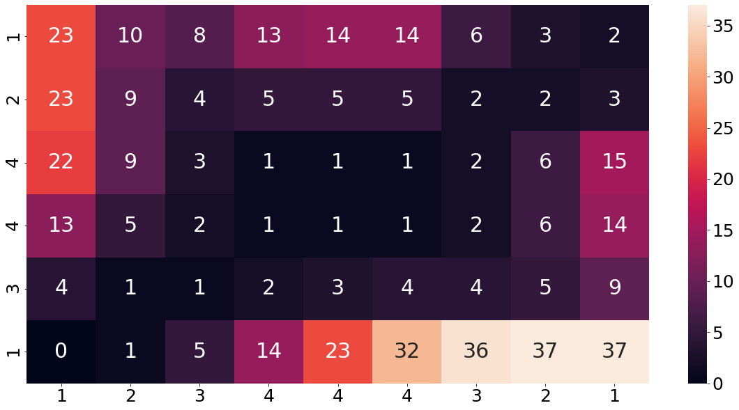
To make that concept a bit clearer, let us consider another example. The value 9 in the third row from the top and second column from the left was calculated in the following way. We start by taking a look what the base-cost matrix is at this position. From the cost matrix above, we find that the base-cost at this point is a four. Now we find the minimum value from all adjacently backward values , which is a five. Summing those two values up, leads us to nine.

The last step of calculating the DTW is now to find the optimal warping path which results in the lowest accumulated cost when walking from the lower left to the upper right of the distance matrix. As mentioned earlier, finding such a path must follow certain restrictions which we outlined earlier.

In the following we are using the Python implementation fastdtw, to calculate and visualize the optimal warping path.

dtw_distance, warp_path = fastdtw(array1, array2, dist=euclidean)
cost_matrix = compute_accumulated_cost_matrix(array1, array2)

fig, ax = plt.subplots(figsize=(12, 8))
ax = sns.heatmap(cost_matrix, annot=True, square=True, linewidths=0.1, cmap="YlGnBu", ax=ax)
ax.invert_yaxis()
path_x = [p[0] for p in warp_path]
path_y = [p[1] for p in warp_path]
path_xx = [x+0.5 for x in path_x]
path_yy = [y+0.5 for y in path_y]
ax.plot(path_xx, path_yy, color='blue', linewidth=3, alpha=0.2)
plt.show()

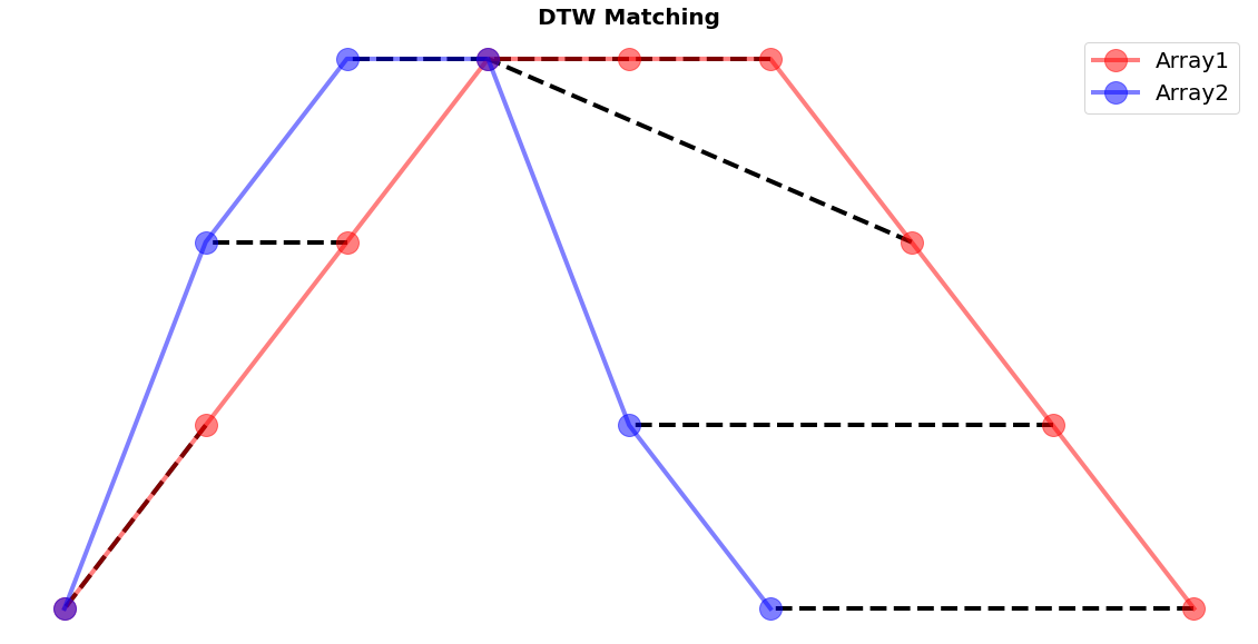
Furthermore, the package also has that capability of plotting how the warping path matching translates into the matching of the individual elements of the two sequences. Through the small snippet of code we get an impressive and intuitive idea how each element is compared to a counterpart of the other series.

fig, ax = plt.subplots(figsize=(20, 10))
fig.patch.set_visible(False)
ax.axis('off')
for [map_x, map_y] in warp_path:
    ax.plot([map_x, map_y], [array1[map_x], array2[map_y]], '--k', linewidth=4)
ax.plot(array1, color="red", marker="o", label="Array1", linewidth=4, markersize=20, alpha=0.5)
ax.plot(array2, color="blue", marker="o", label="Array2", linewidth=4, markersize=20, alpha=0.5)
ax.set_title("DTW Matching", fontsize=20, fontweight="bold")
ax.legend()
plt.show()

It is important that the concept of the distance-matrix is clear to the reader. In case a more visual explanation is desired, we recommend the following tutorial video.

Warping Band

Of course not all time-series are as short as the two example sequences we used above. Especially audio data can be reach extensive lengths. When considering the finding of the optimal warping path from above, it quickly becomes a daunting task to find the optimal warping path with that many possibilities. In order to limit the amount of possibilities, and for making the problem computationally feasible, the window-size parameter is introduced. This parameter was already mentioned as the fourth restrictions from the original paper. In practice this window parameter looks like the following:

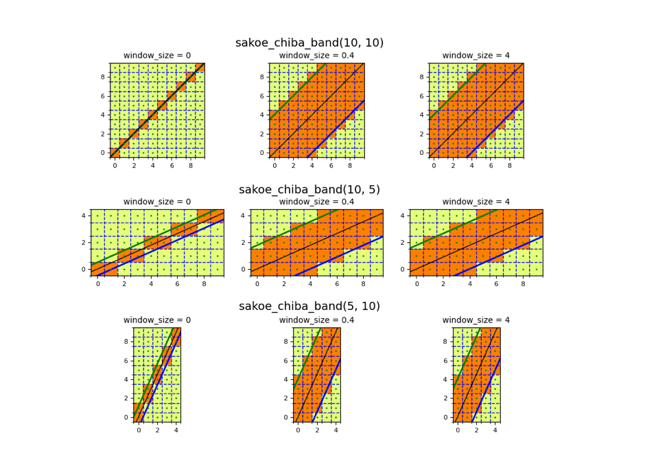Source: https://pyts.readthedocs.io/en/stable/auto_examples/metrics/plot_sakoe_chiba.html#sphx-glr-auto-examples-metrics-plot-sakoe-chiba-py

As visible from the charts above, we can see that by cutting off the upper left and lower right corner, the amount of possibilities goes down drastically. The size of this window parameter is a hyper-parameter set by the user. Hence, every time we are writing about a relative band size, we are referring to this concept.

Implementation of DTW in Python

Given how powerful this algorithm is and the fact that this concept was not discovered yesterday (the original paper published in 1981), one would think that there is a commonly agreed code implementation in Python of that algorithm. For many years that was also the case and it was called fastdtw, implemented by Salvador, Stan and Chan Philip [2]. Their implementation was and still is wildly popular and used in much of academic’s work. In fact, this post initially also used fastdtw for everything upcoming.

The appeal of fastdtw is, as its name already suggests, it is fast. It does that by approximating the true value of the warping path instead of trying to calculate the true value itself. That is done through a combination of three steps, called: Coarsening, Projection and Refinement. What these three steps do is to first shrink the original time-series into a smaller one, find the optimal warping path using the smaller version and then scale it back to the original size. In order to make that rescaling more accurate, we then refine the warping path with superior matches within a neighborhood of the projected path. The size of this neighborhood is determined by the parameter radius which represents a hyper-parameter of the fastdtw implementation.

Nearly at the end of this writing this post, we then found a relatively new (2020) paper with the edgy title FastDTW is approximate and Generally Slower than the Algorithm it Approximates, written by Renjie Wu and Eamonn J. Keogh (they are both very interesting people who’s personal websites are worth to taking a look at). From this title it is already clear that this paper is not here to make any friends. They even conclude their impressive piece of work by stating a quote of an academic who used the fastdtw implementation and found more accurate and faster results when using the implementation of Wu and Keogh. Since they did us the honor and made their Python implementation public, we are using their implementation in the following.

For the rest of this post we are using the implementation by Wu and Eamonn with a slight addition in order to be able to compare time-series of different lengths. Namely, we are padding the shorter series to reach the length of the longer one.

def adjust_length(longer_array, shorter_array):
    """ Pad the smaller series in order to have the same length as the longer array
    :param longer_array: the longer of the two sequences
    :param shorter_array: the shorter of the two sequences
    :return: the padded shorter sequences, which now has the same length as the longer array
    """

    difference_in_length = len(longer_array) - len(shorter_array)
    padding_zeros = np.zeros(difference_in_length)
    adjusted_array = np.concatenate([shorter_array, padding_zeros])
    return adjusted_array

def dtwupd(a, b, r):
    """ Compute the DTW distance between 2 time series with a warping band constraint
    :param a: the time series array 1
    :param b: the time series array 2
    :param r: the size of Sakoe-Chiba warping band
    :return: the DTW distance
    """

    if len(a) < len(b):
        a = adjust_length(longer_array=b, shorter_array=a)
    else:
        b = adjust_length(longer_array=a, shorter_array=b)

    m = len(a)
    k = 0

    # Instead of using matrix of size O(m^2) or O(mr), we will reuse two arrays of size O(r)
    cost = [float('inf')] * (2 * r + 1)
    cost_prev = [float('inf')] * (2 * r + 1)

    for i in range(0, m):
        k = max(0, r - i)

        for j in range(max(0, i - r), min(m - 1, i + r) + 1):
            # Initialize all row and column
            if i == 0 and j == 0:
                c = a[0] - b[0]
                cost[k] = c * c

                k += 1
                continue

            y = float('inf') if j - 1 < 0 or k - 1 < 0 else cost[k - 1]
            x = float('inf') if i < 1 or k > 2 * r - 1 else cost_prev[k + 1]
            z = float('inf') if i < 1 or j < 1 else cost_prev[k]

            # Classic DTW calculation
            d = a[i] - b[j]
            cost[k] = min(x, y, z) + d * d

            k += 1

        # Move current array to previous array
        cost, cost_prev = cost_prev, cost

    # The DTW distance is in the last cell in the matrix of size O(m^2) or at the middle of our array
    k -= 1
    return cost_prev[k]

Audio Files - Numbers

As already mentioned earlier, the concept of Dynamic-Time-Warping was originally invented for sound research. Sound can be seen as a time-series given that it represents nothing other than pressure over time.

To assess the performance of the Python implementation of DTW, I recorded myself saying the three words “one”, “two” and “three” in five different speed levels, resulting in 15 audio files. The following function and output below gives an idea how that would sound like. More explicitly, we are showing the medium-speed and quick version of saying the word “one”.

Note that because of the default .m4a format of QuickTimePlayer, we had to first change the format of the sound file before we can display the audio file. Furthermore, it was not possible to loop the displaying of the sound-files, which is the reason of using two cells in the following.

def show_audio(m4a_path):
    m4a_file = AudioSegment.from_file(m4a_path)
    wav_file = "../wav.wav"
    m4a_file.export(wav_file, format="wav")
    file = ipd.Audio(wav_file, rate=22050)
    os.remove(wav_file)
    return file

show_audio(f"{DATA_PATH}/numbers/one_1.m4a")

show_audio(f"{DATA_PATH}/numbers/one_5.m4a")

The experiment we are aiming for is to see how much better the DTW distance is compared to the euclidean distance, when it comes to clustering same words together. For that we starting by defining a couple of functions, namely a function to load one sound file at a time, as well as one function which loops through all files within one folder. Note that we are normalizing the sound sample, given that are not interested for this experiment to be influenced by how loud a word was said.

def load_audio_file(audio_path):
    audio = AudioSegment.from_file(audio_path)
    audio = audio.set_frame_rate(SAMPLING_RATE)
    samples = np.array(audio.get_array_of_samples())
    normalized_samples = samples / max(samples)
    return normalized_samples

def load_sound_data(folder_name):
    folder_path = f"{DATA_PATH}/{folder_name}"
    file_names = os.listdir(folder_path)
    list_audio_arrays = {i: load_audio_file(f"{folder_path}/{i}") for i in file_names
                         if i.endswith("m4a") or i.endswith(".mp3")}
    return dict(sorted(list_audio_arrays.items()))

Sampling rate

One particularly important aspect when it comes to sound data is the sampling rate. The sampling rate defines the number of samples per second taken from the continuous signals “sound” in order to make it discrete and measurable. This rate is measured in hertz (Hz) per second. Usually audio signals have a sampling rate of 48.000, which is the standard audio sampling rate used by professional video equipment.

The problem that comes with a higher sampling rate is that we are getting more data. The sound is richer. Normally we would think that this is positive and desirable. This might be true when listening to music, but it is not as desirable when trying to work with sound-data. Since DTW already suffers from heavy scaling issues (which was the main motivation of fastdtw), we are not interested in getting so much data.

When processing sound-data, it is not necessary to sample anywhere close to the standard 48,000 Hz. In the following we are using a sampling rate of 100 Hz, which is the usual sampling rate for sound-data.

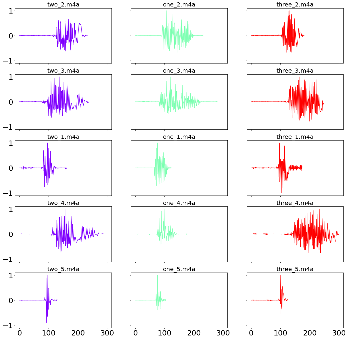
Visualizing of sound-waves: Numbers

In the following we define two functions in order to find all the audio-files in a local directory, as well as loading each individual file, changing the sampling rate and standardize the resulting numpy array between zero and one. From the chart below we can nicely see that the fifth recording, which was designed to be a fast-pace version of the word, is on average much shorter than the other recordings.

# Load data
SAMPLING_RATE = 100
numbers_sound_dict = load_sound_data("numbers")

# Plotting the different numbers
number_names = list(set([i.split("_")[0] for i in numbers_sound_dict.keys()]))
extension_names = list(set([i.split("_")[1] for i in numbers_sound_dict.keys()]))
NUMBER_OF_NUMBERS = len(number_names)
NUMBER_OF_FILES_PER_NUMBER = len(extension_names)

fig, axs = plt.subplots(ncols=NUMBER_OF_NUMBERS, nrows=NUMBER_OF_FILES_PER_NUMBER, sharex="all", sharey="all",
                        figsize=(20, 20))

color= cm.rainbow(np.linspace(0, 1, NUMBER_OF_NUMBERS))
for j, (c, number) in enumerate(zip(color, number_names)):
    for i, example in enumerate(extension_names):
        key_name = f"{number}_{example}"
        axs[i, j].plot(numbers_sound_dict[key_name], color=c)
        axs[i, j].set_title(key_name)
plt.show()

It is now time to compare the performance between the two distance algorithms. This is done comparing every recording against the “one_1.m4a” recording. A good performing distance algorithm would then be able to find a smaller distance between every version of “one”, compared to recordings of the words “two” or “three”.

relative_warping_band = 5 / 100
array1 = numbers_sound_dict["one_1.m4a"]
euclidean_df = pd.DataFrame(np.empty((NUMBER_OF_FILES_PER_NUMBER-1, NUMBER_OF_NUMBERS)),
                            columns=number_names, index=range(2, NUMBER_OF_FILES_PER_NUMBER+1))
dtw_df = euclidean_df.copy()
r = int(len(array1) * relative_warping_band)

for i, sample in enumerate(tqdm(range(2, NUMBER_OF_FILES_PER_NUMBER+1))):
    list_euclidean, list_dtw = [], []
    for number in number_names:
        array2 = numbers_sound_dict[f"{number}_{sample}.m4a"]
        euclidean_df.loc[sample, number] = euclidean_distance_calculator(array1, array2)
        dtw_df.loc[sample, number] = dtwupd(array1, array2, r)

100%|██████████| 4/4 [00:00<00:00, 80.13it/s]

Before comparing the results we are scaling the distances for better readability. It is important to note that it is not possible to compare distances between algorithm. One cannot say that the distance of the euclidean distance is half the distance of the DTW and therefore shorter. One should only compare distances within the same category. Hence, we are checking in each row which is the smallest distance to the benchmark recording, and then conclude what, according to the algorithm, is the closest match.

def plotting_standardized_results(dataframe, title=""):
    standardized_df = dataframe / np.max(np.max(dataframe))
    cmap = sns.diverging_palette(133, 10, as_cmap=True)
    fig, axs = plt.subplots(figsize=(30, 10))
    sns.heatmap(standardized_df, annot=True, cmap=cmap, ax=axs)
    axs.set_title(title)
    plt.show()
plotting_standardized_results(dtw_df, "DTW")
plotting_standardized_results(euclidean_df, "Euclidean")

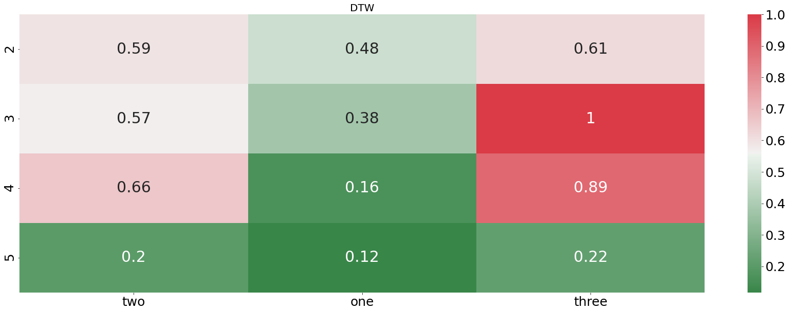
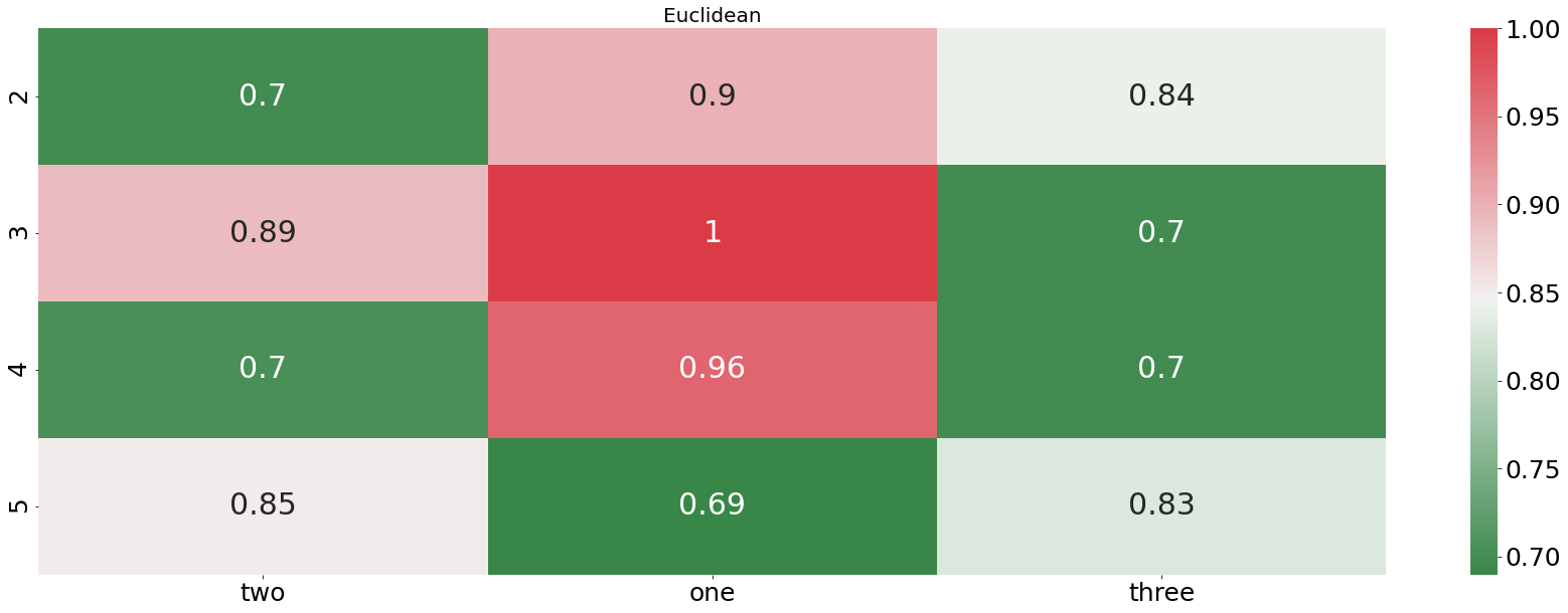
From the plot above we see that the DTW distance is finding pretty accurately which audio file is describing the word “one”. In every example, the DTW distance is finding the right recording. In contrast to that, the euclidean distance is doing horribly, not even finding one correct match. Let us now check how our algorithm is performing when we feed it an entire sentences instead of only one word.

Audio Files - Sentences

For this task I recored two different sentences, which are both inspired by the usage of my Echo Dot. The first recording says: “Please, play the previous song”, whereas the second recording says: “Please, tell me the news”.

Then I took the first sentence, created copies and adjusted the playback speed. I created two faster version, which are played in 0.8x and 0.9x of the time, as well as creating two slower versions, which are played at 1.1x and 1.2x of the original time.

In the following we can take a listen of how that would sounds like:

show_audio(f"{DATA_PATH}/sentences/00_sentence_1x.m4a")

show_audio(f"{DATA_PATH}/sentences/01_sentence_0.5x.m4a")

show_audio(f"{DATA_PATH}/sentences/02_sentence_2x.m4a")

show_audio(f"{DATA_PATH}/sentences/03_sentence_1.5x.m4a")

show_audio(f"{DATA_PATH}/sentences/04_2sentence.m4a")

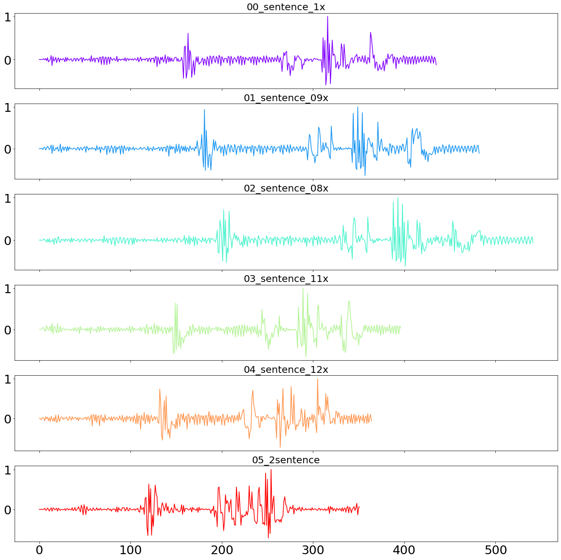
To get an even better feeling of the data, we also take a look at the sound-waves. Note how faster versions of the sentence show a shorter sound-wave, and slower versions a longer wave than the original. The goal of the algorithm is now going to be to connect the identifying characteristics of the time-series, even though they are not happening at the same time anymore.

Just as a side note: If we were to use the standard sampling rate of 48.000 Hz, our time series of that four second long recording would have a length of over 250k observations. An incredibly high amount for such a short recording. Since we do not need that amount of detail of the sound at hand, we are using a sampling rate of 100 Hz.

# Load data
sentences_sound_dict = load_sound_data("sentences")

# Plotting the sentences
def plot_sound_waves(sound_dict):
    NUMBER_OF_SENTENCES = len(sound_dict.keys())
    fig, axs = plt.subplots(nrows=NUMBER_OF_SENTENCES, figsize=(20, 20), sharex="all")
    axs = axs.ravel()
    color= cm.rainbow(np.linspace(0, 1, NUMBER_OF_SENTENCES))
    for i, (c, name) in enumerate(zip(color, sound_dict.keys())):
        axs[i].plot(sound_dict[name], color=c)
        axs[i].set_title(name.split(".")[0])
    plt.show()
plot_sound_waves(sentences_sound_dict)

Now it is time to see how well the DTW method can classify these recordings. A perfect clustering algorithm would show a relatively small distance between the speed-adjusted sentences and the original sentence, and a large distance to the second sentence.

def benchmarking(sound_dict, relative_warping_band):
    benchmark_sound = list(sound_dict.values())[0]
    comparison_names = list(sound_dict.keys())[1:]
    number_of_comparisons = len(comparison_names)
    results_df = pd.DataFrame(np.empty((number_of_comparisons, 2)), columns=["Euclidean", "DTW"],
                              index=comparison_names)
    r = int(len(benchmark_sound) * relative_warping_band)

    for name in tqdm(comparison_names):
        comparison_sound = sound_dict[name]
        euclidean_value = euclidean_distance_calculator(benchmark_sound, comparison_sound)
        dtw_value = dtwupd(benchmark_sound, comparison_sound, r)
        results_df.loc[name, "Euclidean"] = euclidean_value
        results_df.loc[name, "DTW"] = dtw_value
    plotting_standardized_results(results_df)

relative_warping_band = 50 / 100
benchmarking(sentences_sound_dict, relative_warping_band)

100%|██████████| 5/5 [00:00<00:00,  6.79it/s]

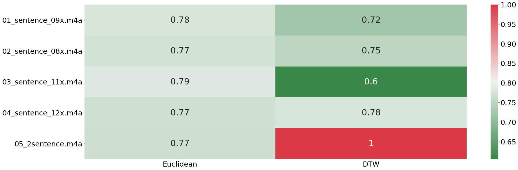
From the plot above we can see that the euclidean distance is not finding any difference in any of the provided tracks. That result is in stark contrast to what the DTW finds. Here we the biggest difference is found with sentence number two (the fifth recording). This results shows impressively how well DTW works even with entire sentences.

Audio Files - Songs

After testing the DTW algorithm on words as well as entire sentences, we now try something even more ambitious. Namely, we are trying to match entire songs. For that purpose we are using two songs from the Arctic Monkeys, namely Arabella and Do I Wanna Know. For the former song we import the live as well as the studio version. Given copyright reasons we are probably better off not playing these songs here, but rather link to the youtube videos we used for the audio files.

• Arabella - Studio Version
• Arabella - Live Version
• Do I Wanna Know - Live Version

song_sound_dict = load_sound_data("songs")
plot_sound_waves(song_sound_dict)

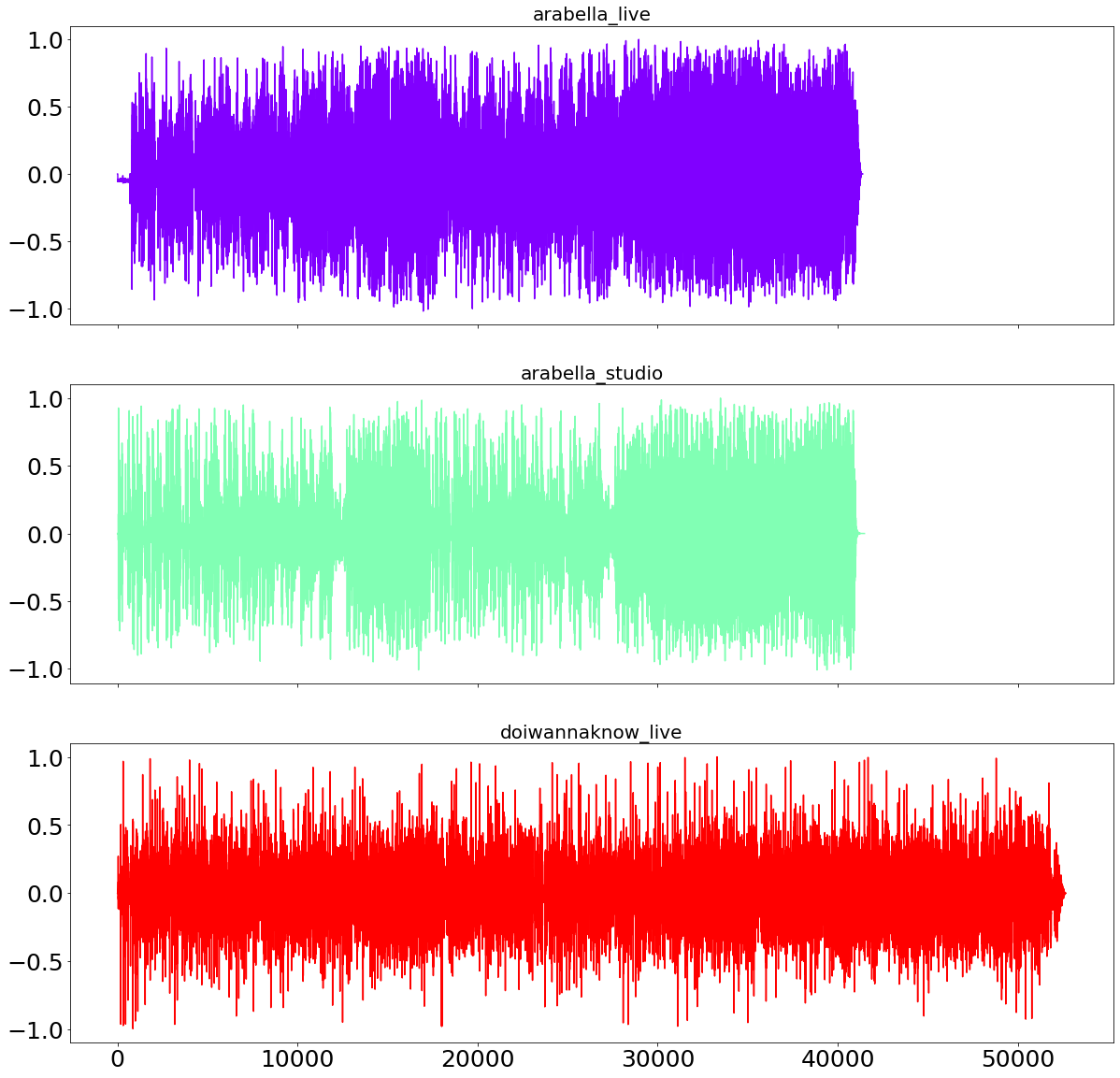
We are now using the live version of Arabella as the benchmark song and calculate the distance between the other two sound-files to the benchmark. As from the sound-waves above visible, even with sampling with a rate of 100Hz, the files are still quite long which will slow down our processing speed.

relative_warping_band = 1 / 100
benchmarking(song_sound_dict, relative_warping_band)

100%|██████████| 2/2 [06:06<00:00, 183.28s/it]

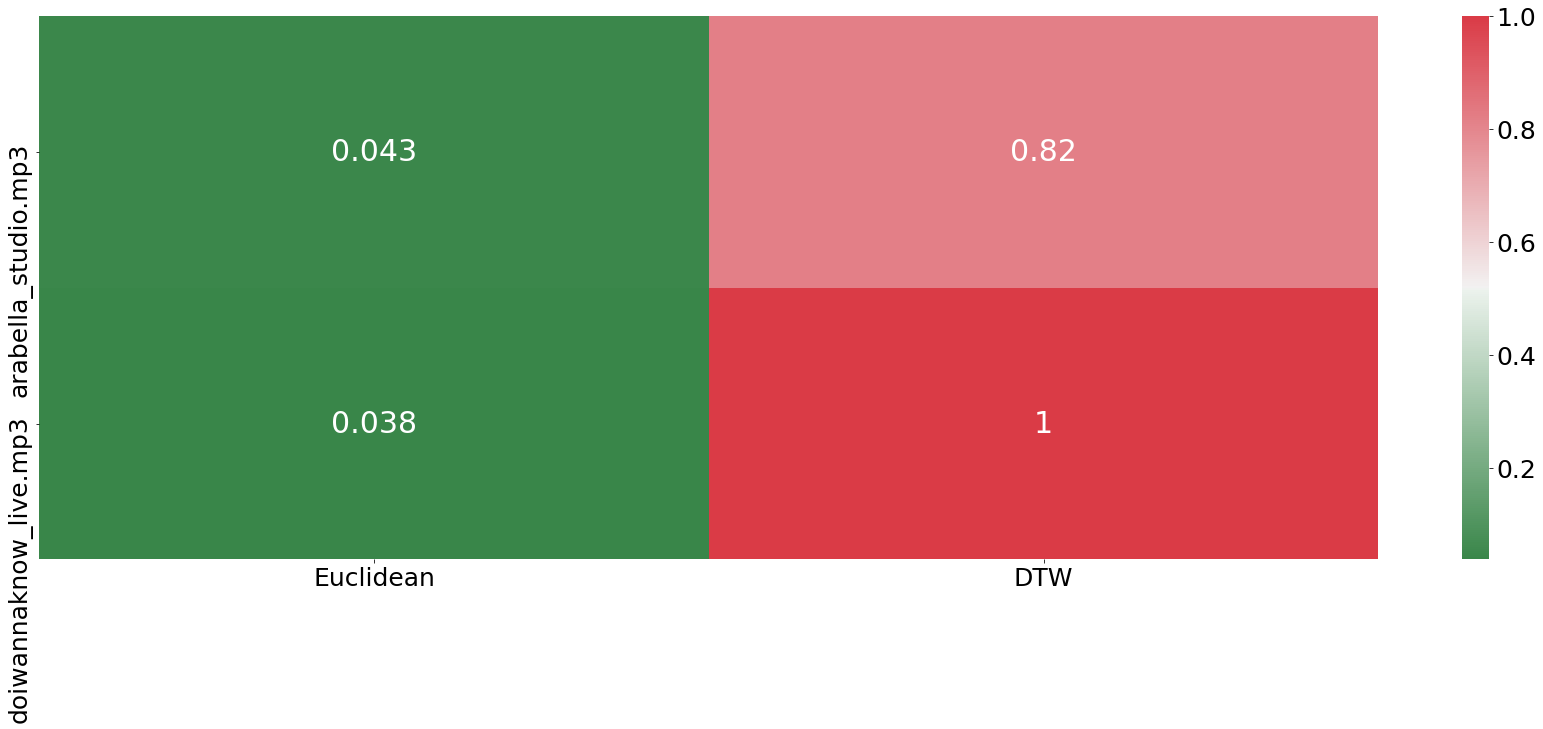
It is important to not get confused about the results above. Even though the euclidean distance measure is shown in green, its performance was very bad, as it shows a closer distance to the different song. In contrast to that, the DTW algorithm was able to find bigger similarities between the studio version of Arabella and the live performance compared to the other song.

Testing two songs of course is not statistically significant by any means, but it shows that we are already going in the right direction.

Nevertheless, all results until now show that the DTW distance measurement is showing fantastic results when it comes to audio-data. It is now time to see whether it can also provide the same benefits for tabular data.

Time Series

Last but not least we are testing the DTW framework for tabular time-series data. Here we are aiming to do time-series classification. Of course, DTW is not able to classify time-series data on its own, since it is merely a tool to assess similarities. Though, when used in combination with a K-Nearest-Neighbors (KNN) algorithm, DTW can serve as a powerful tool to identify the most relevant neighbors.

Data

For this challenge we are using the web traffic time series data from Kaggle. This dataset describes the number of visits to a various websites (shown in the rows) over time (shown in the columns).

NUMBER_ROWS = 500
file_path = f"{DATA_PATH}/time_series/train_1.csv"
data = pd.read_csv(file_path, nrows=NUMBER_ROWS)
data.head()

	Page	2015-07-01	2015-07-02	2015-07-03	2015-07-04	2015-07-05	2015-07-06	2015-07-07	2015-07-08	2015-07-09	...	2016-12-22	2016-12-23	2016-12-24	2016-12-25	2016-12-26	2016-12-27	2016-12-28	2016-12-29	2016-12-30	2016-12-31
0	2NE1_zh.wikipedia.org_all-access_spider	18.0	11.0	5.0	13.0	14.0	9.0	9.0	22.0	26.0	...	32.0	63.0	15.0	26.0	14.0	20.0	22.0	19.0	18.0	20.0
1	2PM_zh.wikipedia.org_all-access_spider	11.0	14.0	15.0	18.0	11.0	13.0	22.0	11.0	10.0	...	17.0	42.0	28.0	15.0	9.0	30.0	52.0	45.0	26.0	20.0
2	3C_zh.wikipedia.org_all-access_spider	1.0	0.0	1.0	1.0	0.0	4.0	0.0	3.0	4.0	...	3.0	1.0	1.0	7.0	4.0	4.0	6.0	3.0	4.0	17.0
3	4minute_zh.wikipedia.org_all-access_spider	35.0	13.0	10.0	94.0	4.0	26.0	14.0	9.0	11.0	...	32.0	10.0	26.0	27.0	16.0	11.0	17.0	19.0	10.0	11.0
4	52_Hz_I_Love_You_zh.wikipedia.org_all-access_s...	NaN	NaN	NaN	NaN	NaN	NaN	NaN	NaN	NaN	...	48.0	9.0	25.0	13.0	3.0	11.0	27.0	13.0	36.0	10.0

5 rows × 551 columns

Given that we are only show-casing DTW, and considering how computational expensive DTW is, there is no reason for importing more than 500 observations. We start by replacing missing observations by a zero, as it is suggested on the Kaggle website. Afterwards we drop the page name, since it does not contain any meaning to us.

data.fillna(0, inplace=True)
data.drop(columns=["Page"], inplace=True)

Quite importantly for our example is the creation of a binary target variable, since as of now, every cell contains a integer variable. Given that we would like to show an example of binary classification, we take the last column (which is also the last date) and turn in into a binary variable. This is done by replacing every number above the median number of hits of that day with True and everything below the median with False.

Last, but not least we are dividing the data into train and test, in order to find a representative performance measure. We are holding out 20% test-data as well as setting the random-state to 42 in order to ensure the reproducibility of our results.

last_column_name = data.columns[-1]
X, y = data.drop(columns=last_column_name), data.loc[:, last_column_name]
bool_y = y > np.median(y)
X_train, X_test, y_train, y_test = train_test_split(X, bool_y, train_size=0.8, random_state=42)

We are then trying to classify this binary target variable through a KNearestNeighbor model, which uses the DTW distance to find surrounding neighbors. For comparison reasons, we are benchmarking the performance of using the DTW distance, by including the euclidean distance as well.

For doing that we are using the handy implementation from tslearn, which provides us with the class KNeighborsTimeSeriesClassifier. This class has the option to specify which kind of distance we would like to use for finding the nearest neighbor.

params = {"n_neighbors": [5, 15, 30, 50]}
pred_dict = {}
metrics = ["dtw", "euclidean"]
for metric in metrics:
    estimator = clone(KNeighborsTimeSeriesClassifier(metric=metric, n_jobs=-1))
    clf = GridSearchCV(estimator=estimator, param_grid=params, n_jobs=-1)
    clf.fit(X_train, y_train)
    y_pred = clf.best_estimator_.predict(X_test)
    pred_dict[metric] = y_pred

Before looking at the results of our classifiers, we also prepare a more challenging competitor to the DTW algorithm, namely GradientBoostingClassifier.

metrics.append("gb")
gb_model = GradientBoostingClassifier()
gb_model.fit(X_train, y_train)
pred_dict["gb"] = gb_model.predict(X_test)

To get a good overview about the performance of all classification methods, we are using a bunch of performance metrics.

performance_evaluation_dict = {
    "accuracy": accuracy_score,
    "precision": precision_score,
    "recall": recall_score,
    "f1": f1_score
}

evaluation_df = pd.DataFrame(np.empty((len(performance_evaluation_dict), len(metrics))), columns=metrics,
                             index=performance_evaluation_dict.keys())
for metric in metrics:
    for key, value in performance_evaluation_dict.items():
        score = value(y_test, pred_dict[metric])
        evaluation_df.loc[key, metric] = score
fig, axs = plt.subplots(figsize=(10, 10))
sns.heatmap(evaluation_df, annot=True, ax=axs)
plt.show()

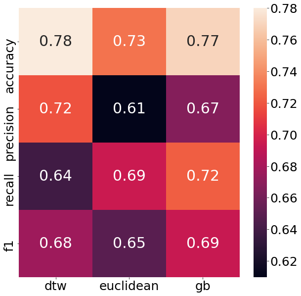
As can be seen from the chart above, the DTW nearest neighbor shows an impressive performance. Not only does it beat the euclidean distance measure in every performance metric, it even beats the GradientBoostingClassifier in half of all categories. That is a big deal, given that in the end it is still K-Nearest-Neighbors what is run under the hood. The neighbors which are chosen through the DTW method, though seem to quite helpful to figure out the structure of the target variable.

All in all the DTW distance measurement is a powerful tool in order to enhance time-series classification in all areas. One has to be aware of the bad scaling issues, as this algorithm can become computationally expensive real quick.

Appendix

• [1] Sakoe, Hiroaki, and Seibi Chiba. “Dynamic programming algorithm optimization for spoken word recognition.” IEEE transactions on acoustics, speech, and signal processing 26.1 (1978): 43-49.
• [2] Salvador, Stan, and Philip Chan. “Toward accurate dynamic time warping in linear time and space.” Intelligent Data Analysis 11.5 (2007): 561-580.
• [3] Wu, Renjie, and Eamonn J. Keogh. “FastDTW is approximate and Generally Slower than the Algorithm it Approximates.” IEEE Transactions on Knowledge and Data Engineering (2020).