Various techniques on dealing with multi-output classification

This post evaluates different approaches when facing a multi-output within a classification problem. A multi-output describes a combination of several outputs put together. For example, a multi-output would describe a situation in which the classification model would not only have to predict whether the image shows a dog or a cat, but also which color the animal is.

There are two main approaches for this problem. We could either split this task into multiple single-classification models, in which each model outputs exactly one attribute. The alternative would be to use exactly one model which was designed to handle a multi-output in the first place. This post applies both methods on a scraped dataset in order to shed some light on the question when to go for which approach.

The entire code-base for this project can be found here.

Data

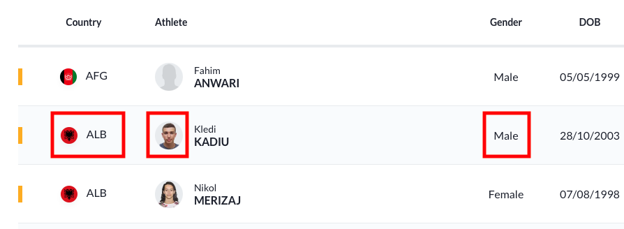
Instead of taking a pre-made image dataset, we scraped the meta information and images of the athletes participating in the water disciplines of the Tokyo 2020 Olympics. As the image below shows us nicely, the database contains information about the country the athlete is participating for, as well as the gender of the person (information in the red squares). The decision for this website was made given the good data quality (e.g. all athletes were shot from the same angle) as well as the (okayish) amount of images of people. The image below also shows a case in which we no image of the athlete was provided (first athlete). In these situation we disregarded the information altogether.

After scraping the meta information from the website, we made one small addition to our dataset, namely the inclusion of the continent information. That is because we preferred to predict the continent attribute of an athlete rather than the country. The main reason for this decision was the limited amount of images we have for each country. In total we were able to scrape around 1.000 images of athletes with their meta information attached. Given that we have 196 official countries on earth, predicting each country separately would have resulted in approximately (1000 // 196) five images for each country (assuming that it is evenly distributed). That amount is way too little for training an image classification model, even when using the power of transfer learning. We therefore decided to map every country to the six continents: Europe, Africa, Oceania, South America, North America and Asia (sadly no athlete is from Antarctica).

Adding the information of the athlete’s continent sounds easier than it turned out to be. That is because of the country information provided on the website we scraped our data from. As it can be seen from the image above, the website provides us with a three letter country-code. More specifically the country-code provided on the website is a so-called National Olympic Committee (NOC) country-code. The issue with this country code is, that it is rarely used anywhere other than the Olympics. Therefore, there are pretty much no mapping tables to translate NOC country-codes to continents. In order to still do so, we first mapped the NOC country-codes to more well known country-codes, such as ISO 3166. This mapping was done by scraping the mapping table from a third-party website. Afterwards we made use of the handy Python package pycountry_convert in order to map the ISO code to the continent specification. The table below shows the final result of the meta information we collected from the website. One notes that we also translated the date of birth to the actual age, using November 2021 as the reference date.

import pickle
file = open("../data/processed/general/meta_df.pickle", "rb")
pickle.load(file).head()

	number	country_code	sports	gender	age	continent
0	1	ALB	Swimming	Male	17.996263	Europe
1	2	ALB	Swimming	Female	23.220189	Europe
2	3	ALG	Open Water	Female	32.707037	Africa
3	4	ALG	Swimming	Female	28.055333	Africa
4	5	ALG	Swimming	Male	29.232633	Africa

Data Imbalance

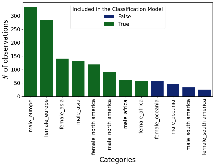
Before moving to the actual classification modeling, we have to check the class imbalance in our data, in order to adjust for potential imbalances. That is necessary, since when a classification model overly sees one class (a.k.a majority class) compared to another (a.k.a minority class), it fails to learn and understand the distinguishing factors between these two classes. From the chart below, we can see that there is quite a bit of imbalance in the data. Furthermore, the two continents Oceania and South America have so few observations, that we decided to drop these two continents, as the amount of images is too low relative to the other classes.

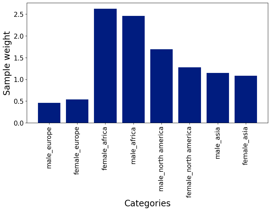
One valid form of countering a class-imbalance within a classification problem is to adjust the sample weight for each of the priorly selected categories. This weight makes the model understand the severity of getting a certain observation wrong. Predicting an observation incorrectly which has a higher weight impacts the model’s training much more, than misclassifying an observation from the majority class. In the following chart, we can see that the weight is quite low for European observations, but quite high for African observations. That is because the class weight is inversely related to the amount of observations in the data. Since we have so many observation from Europe, the model should not stress so much about getting all of them right, but since we have so few African observations, the model should really pay attention to those ones.

In order to get a better feeling of how difficult this classification task is, we should take a look at our observations. In the following we show example images from all eight categories. There are eight categories, since we are dealing with all possible combinations of two genders and four continents. This information about the length of the output space, is also important to know, as it allows to approximately (since it does not account for imbalance) calculate what performance a random classification model would achieve, namely 1/8 = 12.5%.

Furthermore, the images below give us a good indication of how difficult the task at hand is. This is especially visible when comparing the visual appearance people from North America and Europe. Since both continents have a high amount of white people, it is quite difficult to tell them apart. On the other hand, it is not difficult to tell whose male or female. In the following we will see that the model confirms these hypothesis of how difficult which classification is.

Classification Methods

After exploring the data and adjusting the class-imbalance, it is now time to talk about the different possibilities to deal with the multi-output of this classification problem. All methods mainly represent a different way to encode the target label each observation has. This is because machine learning model is unable to make use of the string target: male_europe. We have to encode that target into a numeric format. Of course there are many different methods of how one could do that, three of which are detailed below and applied on our dataset. Regardless of the encoding technique, all encoding mechanisms are then stacked on the pre-trained network VGG16, by using transfer learning. The idea and workings behind transfer learning are out-of-scope for this post but can be learned about in this other post of mine.

Multi-Class

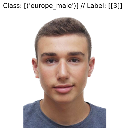
Arguably, the most popular choice is the so-called multi-class handling. A multi-class describes the situation in which we assign each combination of the two outputs an unique id. When for example facing a female person from Asia, we would simply say that this combination is encoded to class 1. A male person from Asia would then be (for example) class 2, and so on. From these two examples, one notices that this approach scales badly. Having n categories in the first output space, and m in the second, would result in $n \cdot m$ combinations.

Another weakness of this approach is that we treat all labels completely different, even though they may have a partial overlap. If for example our classifier predicts male_asia as female_asia, the loss function of the model is unaware that it got 50% of the target labels correct. It treats these two classes as something entirely different. That behavior can of course also have its benefits, namely for tasks in which we classify objects which are fundamentally something else. Herein the behavior of not getting partial credit is also desired. In the following we see an example of this encoding technique.

Multi-Label

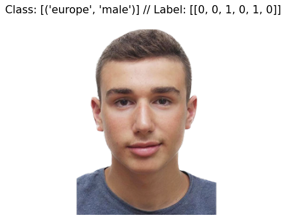
A second viable option is the so-called multi-label option. That method represents a generalization of the multi-class option, in which no constraint is given of how many output classes can be set to true or false. To better illustrate that, let us imagine an output space in which the only two continents from which a participant could come from is Europe or Asia, and that the person’s gender is constraint to Female and Male. In this scenario the output space of a multi-label approach would look the following way:

\[[Bool_{Asia}, Bool_{Europe}, Bool_{Female}, Bool_{Male}]\]

In the equation above Bool represents a boolean, which can be set either true (1) or False (0). Following that logic, a female Asian would therefore be encoded as [1, 0, 1, 0]. This encoding method is strikingly different to the multi-class approach, as multiple outputs can be true. For that reason multi-label encoding is used when it is unclear how many outputs could be shown in the image. If we would face a group photo of a male European and a female Asian, the multi-class encoding technique would have a hard time, whereas the multi-label approach would simply return [1, 1, 1, 1], because all categories are visible on that image.

Given that in our classification exercise we only face images from exactly one person, this type of encoding cannot play its main strength. Though it is still a strong contender, since it is able to learn from interaction effects. That is because if the model predicts male_asia, even though the correct label is female_asia, the classification model understands that it was partially correct. That is the main advantage of the multi-label encoding compared to the multi-class. Furthermore, it scales massively better than the multi-class problem. In a situation in which the two output spaces have the lengths of n and m respectively, then increasing the output space of n by one unit, would increase the total output layer of the multi-label approach by one. In the following we see an example of the multi-label technique:

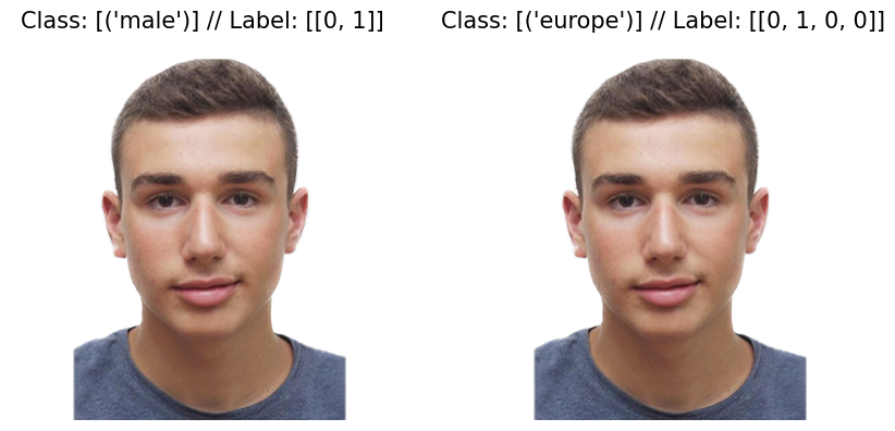
Chained Single Classification

Lastly, another option of how to deal with our multiple-output classification problem is that we break down the problem into several disjoint classification themselves. In our scenario, that would mean that we train a classification model for the person’s gender and continent information separately. In the end we would then hand a new image to the two fitted classification models and retrieve the respective information from each. The first model would for example tell us that the person is Male and the second model would give us the additional information that the person is predicted to be Asian.

The strengths of this approach is that each model can solely focus on one task at once and therefore can potentially achieve a better prediction result on a certain task than any of the previously mentioned models can. Of course, this approach also has its flaws. First of all, we need one model per output category, meaning that this approach is computationally expensive. Second of all, the model cannot use any interaction effects. This can be illustrated through the following example. Let us imagine that females from Asia look fundamentally different than females from other continents. A classification model which solely distinguishes between male and female, without any continent information will have a hard time to understand why it fails so often with female Asians. This is because, this classifier lacks the additional important information that the female is Asian and therefore has to be treated differently than other females. The previously mentioned classification methods though makes use of this additional continent information, and are therefore able to deal with that problem.

In the following we see an example of how an image is encoded when using the chained single classification.

Data Processing and Augmentation

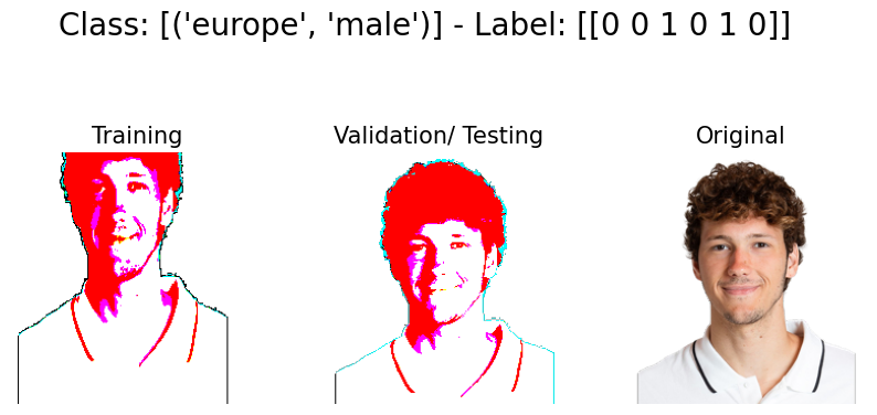
As mentioned earlier, all of the three presented methods are basically nothing other than different ways of how to encode the multi-output target. All three approaches though are of course not enough to classify the image itself. One needs an underlying Convolutional network to do the main work. Within all kinds of image classification tasks, it is relatively unwise to train a new neural network from scratch, given the extensive amount of pre-trained models available. One condition when using a pre-trained model, is that we are using the same kind of pre-processing of our images, as the pre-trained model used when it was initially trained. From the images below we can nicely see what kind of transformation is applied when comparing the images under the heading “Validation/ Testing” and “Original”.

Another important aspect to consider when having a small image dataset, is the power of data augmentation. Data augmentation describes the process of artificially increasing the amount of data through transforming (augmenting) the already existing database, by e.g. stretching, zooming, flipping the original image. The image under the header “Training” from the figure below shows nicely how the image under the header “Validation/ Testing” was stretched and zoomed. Through these altering of the original images, the model sees quite a bit more different images, than it would if we feed it only the unaltered images. The exact augmentation settings used in this project, can be found in the parameters configuration file on github.

Results

In the following we present and discuss the results of the project. We do that in the following fashion: First we evaluate the results of each approach separately, pointing out the main strengths and weaknesses of each approach and hypothesis on the reasons for that performance. Afterwards, we show a head-to-head comparison of the different approaches and try to shed some light on why a certain approach worked better than others. Lastly, we point out the key-learnings of this project and what could be improved.

Multi-Label

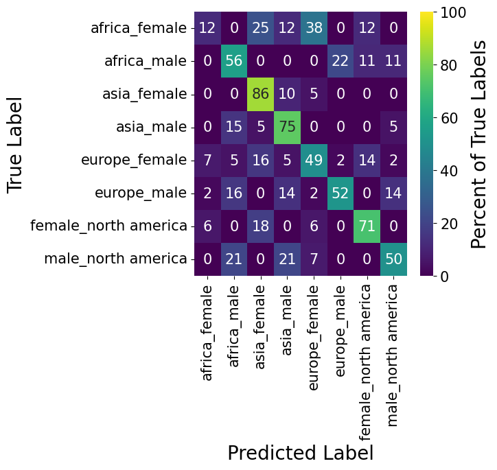
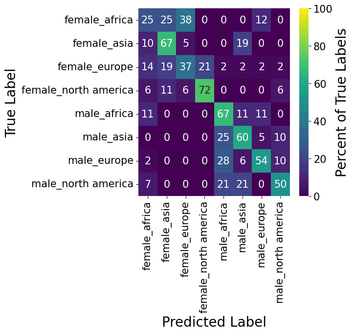
A common method when evaluating a classification model is the so-called confusion-matrix. Each row of that matrix shows one actual target class, whereas the columns show what was predicted by the classification model. A perfect classifier would have all observations along the diagonal of the matrix.

In the following figure we plotted such a confusion matrix for our classification model. In order to showcase the performance a bit better, we slightly tweaked the confusion matrix though. Instead of displaying the absolute amount of observations in each cell, we show the percentage value of the sum of each row. The value in the top left for example tells us that 12% of africa_female were actually classified as africa_female. Two boxes to the right we also find that 25% of africa_female were classified as asia_female. Of course, a perfect result would show 100% along the diagonal of the confusion matrix. It is furthermore to be said that all predictions were made on a hold-out test dataset, which represents 15% of the sub-selected image dataset and therefore represent around 150 images.

As already implicitly noted in the prior example, the performance for africa_female is quite poor. Though, it has to be said that the performance of all categories is at least four times better than for the africa_female category. For all other categories, the algorithm classified on average around 50% or more of the test-images correctly. It is furthermore nicely visible that the misclassification happen mostly along the continent dimension and not on the gender attribute. Taking the europe_female category as an example. Herein we find that 49% of all images of that category are correctly classified as europe_female. The other two larger buckets for that category are asia_female (16%) and female_north america, meaning that the algorithm understood the difference between male and female, though had more problems to understand the continent attribute of that person. The very same phenomena is also visible for the male_north america category. Interestingly, the algorithm had no problem of telling European and North American males apart, but rather to distinguish North American, African and Asian.

The fact that the classification model performs much better along the gender attribute compared to the continent attribute is also understandable. Given the migration flows around the world, it is pretty much impossible to tell with certainty where somebody was born, simply by their appearance. Though, which gender a person is, is easier to tell in comparison.

Overall, the performance of the multi-label approach is rather decent, of course it has its weaknesses along the continent dimension, though as mentioned above, this is also difficult task in general.

In order to shed more light on which observation the algorithm was able to classify, and which one the classifier failed on, we provide some examples below to get a better feeling. On the left side we see all the examples which the classifier was able to predict, whereas the right side shows the failures of our model. By looking at the examples the classifier failed at, it becomes obvious why this is such a difficult classification task.

Multi-Class

Many of the findings of the multi-label classifications also show up during the evaluation of the multi-class metrics. For example, the misclassification also happens mostly on the continent dimension rather than the gender dimension. In a direct comparison with the multi-label classification, we find that the multi-class algorithm performs better than the multi-label approach for 75% (6/8) of the eight categories. That finding suggests that all categories have something quite unique about them and that the inability to recognize partial correctness (e.g. classifying gender correctly, but incorrect continent) does not lead to a superior prediction performance.

It would be quite interesting to see whether this superior performance would also remain if we increase the number of continents and/or introduce another output dimension to the model.

When looking at which samples the multi-class classification model got wrong, we actually find several familiar faces which the multi-label method was also unable to correctly predict.

Independent Single Classification

The assessment of the results for the chained classification can be split up into its individual components. Namely we can directly assess how well the algorithms performed on both dimensions respectively. Since this analysis holds some interesting pieces, we therefore go over the evaluation of both categories one by one.

Gender

The confusion matrix below confirms what we hypothesized already when evaluating the performance of the two previous models. The classification algorithm performs relatively strong along the gender dimension. Most of the predictions are correct, with the algorithm being slightly stronger detecting males (97%) compared to females (89%).

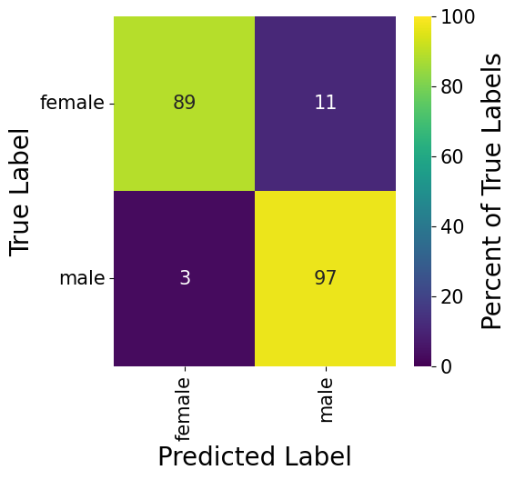
When looking at the examples which the algorithm failed to detect, we see that most observations where that happened are females with a short hair-cut. This does make sense as short hair-cuts are primarily worn by man, and since the algorithm is learning nothing other than statistics, we also expected such behavior of the algorithm. When we are saying that the algorithm learns to understand what gender a person is, it is of course not measuring the Testosterone level of the person, but rather it looks at similarities of the two clusters. Therefore the model is rather detecting whether the person fits more criteria of a male/female person than anything else.

Continent

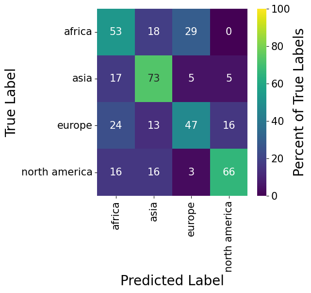
When evaluating the model’s performance along the continent dimension, we have to remind ourselves that the classification happened without any indication of the gender of the person. Meaning that the algorithm would have to ignore the visual differences of the gender and focus only on other features which would indicate the origin of a person.

The result below shows clearly that this task is considerably more difficult than the previous one. For the Europe class, the algorithm even fails on more than half (47%) of its predictions.

Total

Last but not least we take a look at the combination of the two single classification tasks. The confusion matrix is relatively empty in the top right and bottom left corner, showing that there was basically no misclassification on the gender dimension. Though, the disperse top left and bottom right corner show that there was quite a bit misclassification along the continent dimension.

Given that this algorithm performs worse on average than the previous two classification techniques, it seems to be the case that the classification of the continent is significantly enhanced when knowing the gender of the person. That would suggest that there is a significant interaction effect between gender and continent.

Overall Assessment

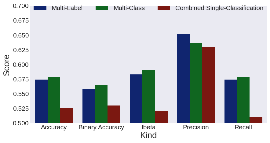
In order to better compare the models head-to-head, we plotted several classification evaluation metrics in the figure below. Herein we see that the multi-class model is slightly ahead of the other two methods for all but one classification criteria. On second place we the see the multi-label model, which manages to outperform the multi-class model in terms of its Precision. That suggests that for some reason the multi-label makes fewer False Positive mistakes. On the disappointing third and last place we find the combined single-classification. This results suggests that failing to incorporate any interaction effects between the gender and continent attribute worsens the overall prediction power of the combination.

Hamming Loss

The figure above has one potentially flaw though which should be mentioned, namely that it fails to award points for a partially correct prediction. That is because of the nature of the target. All three classifiers return in the end a prediction such as male_europe. This very prediction is then compared to the true label. If the true label is male_europe, then we speak of a correct prediction. Though, a male_asia and a africa_female would be both equally incorrect, even though that male_asia is much closer to the truth to the true label than africa_female, where both of the attributes are incorrectly classified.

In order to also attribute partial credit, we have to pick another evaluation metric than the ones we showed in the figure above. All metrics we looked at in the previous figure are commonly used within classification tasks, though when having a multi-output problem, we should also look at something called hamming loss. This loss metric originates from the concept of hamming-distance. Herein we evaluate the number of symbol changes between two strings. For example, the number of symbol changes to go from 010 to 000 is exactly one, namely we change the 1 in the first string to a zero. Changing from 111 to 000 would represent the largest number of symbol changes necessary to change from one string to another.

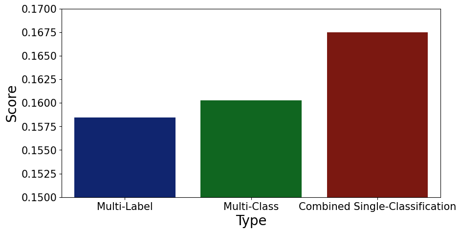
This very method can neatly applied to our prediction problem, since it recognizes that the number of symbol changes between male_europe and male_africa is smaller than between male_europe and female_africa. The figure below shows the results when calculating the hamming loss for all three approaches. One has to remember that we are looking at a loss, therefore a smaller score is better. In contrast to the previous figure, the multi-label approach outperforms the other two. That makes also somewhat sense, as we used a loss somewhat related to hamming loss (binary accuracy) for the training of the multi-label algorithm.

Conclusion

These results lead to quite interesting conclusions. First of all, interaction effects are important. That was particularly visible when looking at the performance of the combined single-classification model. Secondly, whether to use multi-class or multi-label depends heavily what the objective of the classification task is. If we face a black and white scenario, in which a partially correct prediction is worth nothing, then we should use multi-class. If on the other hand, also partial correctness is useful, then we should opt for the multi-label approach. Last but not least. The multi-class algorithm scales the worst. When having a large multi-output space this approach seems likely to fail quicker than the multi-label, which scales considerably better.

Outlook and Improvements

Last but not least we briefly go over several potential improvements to the model performance, if there would have been more time on that project.

Using Chained-Classification instead Independent Combined Classification

One weakness of the combination of two single-classification seems to be the failure of incorporating the gender information when predicting the continent attribute of a person. That seems to be the case given the struggle of the combination classification for the continent attribute. One potential solution for that weakness is the so-called Classifier Chain, as it is described by scikit-learn here. That approach does exactly what it is assumed is missing for our combination prediction. It incorporates the prediction of the previous classifier into the input space of the following classification method. For our example that would mean that we could include the gender information when classifying the continent attribute. Unfortunately, the implementation from scikit-learn does not easily let us use tensorflow with it, which was the reason it was not implemented right away. Though, given the results, this approach could seriously increase the performance of the combination of individual classifiers.

Better & More Images

When looking through the web at other people’s projects of classifying a person’s origin, the datasets people work with are most of the times much cleaner than ours. The projects on the web usually gather and validate their images manually and therefore have much less noise through immigration compared to our dataset, which simply takes the data from the website as a given. It is more than likely that when removing the observations which introduce the noise to our dataset, that we would be more than able to reproduce the classification performance of the other projects on the web.