

NLP with Real Estate Advertisements - Part 1
Analyzing and exploring real estate advertisement descriptions using NLP pre-processing and visualization techniques.
Pre-processing and exploring the text data
Each real estate listing scraped contains a text component, the ad description. The descriptions are actually previews of the full descriptions, scraped from the listing page.
This description text helps to explain what the numbers alone cannot.
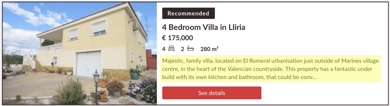
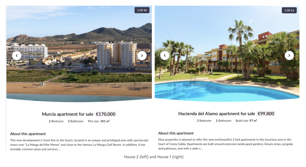
Take for example the following two advertisements, both for houses in the Murcia region of Spain:
House 1: 2 Bedrooms, 2 Bathrooms, Pool, 97m2. Price: €99,800.
House 2: 2 Bedrooms, 2 Bathrooms, Pool, 101m2. Price: €170,000.
How is it possible that House 2 is almost 70% more expensive than House 1? Surely the additional 4 square meters of living space cannot explain that difference. Price differences of such a magnitude with identical feature values make it very difficult for the model to learn.
Looking at the description of each house explains the price difference: House 2 is located directly on the beach. This is important information that will help our model learn to better predict these prices.
After scraping the description preview for all real estate listings, we were left with text samples that looked like this:
- “Amazing villa with incredible views in a very attractive area!\n\nThe view takes you down over the valley, you’ll be able to see Fuengirola and the Mediterranean sea. The house is located on the way from Fuengirola going up to Mijas. \nIt i…”
- ‘This stunning Villa is located on the edge of Almunecar on Mount El Montanes.\n\xa0The location is absolutely stunning with panoramic views of the water / beach, city, mountains. Yes you can look at Salobrena, Motril and Torrenueva.\nThe 2-st…’
- ‘A rare opportunity - a brand new modern villa in a sought after area of lower torreblanca near the beach!\n\nVilla Alexandra is a new modern villa centrally located close to the beach in Torreblanca, Fuengirola. The villa is recently compl…’
- ‘Price Reduction ! Price Reduction ! Now 495.000 euro\n\nThis stunning wooden country house sits on an elevated plot overlooking the village of Alhaurín el Grande with views down the valley and to the Mijas Mountains. The property benefit…’
Our goal is to use the information from this text to help our model predict real estate prices.
Preparing the data for NLP Analysis and Modeling
Before we can extract insights from the text data, we have to prepare the data- getting it into a form that algorithms can ingest and understand.
As we go through these steps, it’s important to keep our goal in mind: what do we want our model to understand from the text? In our case, our goal was to use the description of the real estate advertisement to predict price. At every step of the NLP process, we asked ourselves: will this help our model understand which words have the biggest impact on the price of a house?
The steps taken for analyzing the text data are as follows:
- Tokenize the data
- Lemmatize the data
- Get n-grams
- Visualize
- Repeat
All NLP models and algorithms require the text data to be prepared - usually in a very specific format - before it can be ingested by the model.
Here, we define some NLP terms we’ll be referencing a lot in this section: tokens, documents, and the corpus.
01 Tokenization
Tokenization involves splitting text into its smallest components, called tokens. Tokens are generally words, though they can also be numbers or punctuation marks. The ‘\n’ symbol appearing commonly in the descriptions represents a line break and would also be classified as a token. Tokens are the building blocks that, when combined, give text its meaning.
A document is the entire text for each record, or observation, in our dataset. Each advertisement represents one observation, so each advertisement’s description text is a unique document.
The corpus is the collection of all documents in our dataset.
Nearly every modern NLP library today contains a tokenizer. We used the spaCy package to tokenize the text. In this step, we also removed any tokens representing punctuation or known English stop words.
02 Lemmatization
Once we have the text split into its component tokens, the next step is to make sure these tokens contain as much information as possible for the model to learn from. There are 2 common ways to do this: lemmatization, and stemming. Both lemmatization and stemming are used to reduce words to their root. The idea behind using both of these methods is that the root of the word contains most of the word’s meaning, and that the model learns associations better when explicitly told that words with the same root are essentially the same.
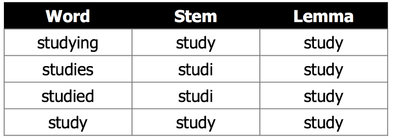
We used lemmatization because it has the advantage of always returning a word that belongs to the language. This makes it easier to read and understand than stem words, especially when the roots are used in visualizations. We also were not concerned about lemmatization taking longer and being more computationally intensive, as our corpus is not extremely large. Lemmatizing the entire corpus took about 10 minutes on a local machine.
03 Creating n-grams
After stemming and lemmatizing the words, we can extract n-grams. N-grams are token groups of n words that commonly appear together in a document or corpus. A unigram is just one single word, a bigram contains 2-word groupings, and so on. N-grams help us quickly identify the most important words and terms in our corpus.
We wanted to see which uni-, bi- and tri-grams were most important in the entire corpus. This is also a great way to quickly visualize our text data and assess how well we’re preparing our description text for our goal of helping the model predict price.
from nltk.util import ngrams
def get_n_grams(processed_docs):
    """
    Getting uni- bi-, and tri-grams from text.
    By default creates grams for entire corpus of text.
    Returns dictionary with {gram_name: gram}
    """
    # initializing list for tokens from entire corpus- all docs
    total_doc = []
    for doc in processed_docs:
        total_doc.extend(doc)
    # extracting n-grams
    unigrams = ngrams(total_doc, 1)
    bigrams = ngrams(total_doc, 2)
    trigrams = ngrams(total_doc, 3)
    # getting dictionary of all n-grams for corpus
    gram_dict = {
        "Unigram": unigrams,
        "Bigram": bigrams,
        "Trigram":trigrams}
    return gram_dict
04 Visualizations
Once we extracted our n-grams, we visualized which words were the most important. We looked at these visualizations through a critical lens and asked, “are these words helping our model learn to estimate price? How can they better support our model’s understanding?”
Below are the initial n-gram plots, plotted with words from the entire corpus of advertisement descriptions.
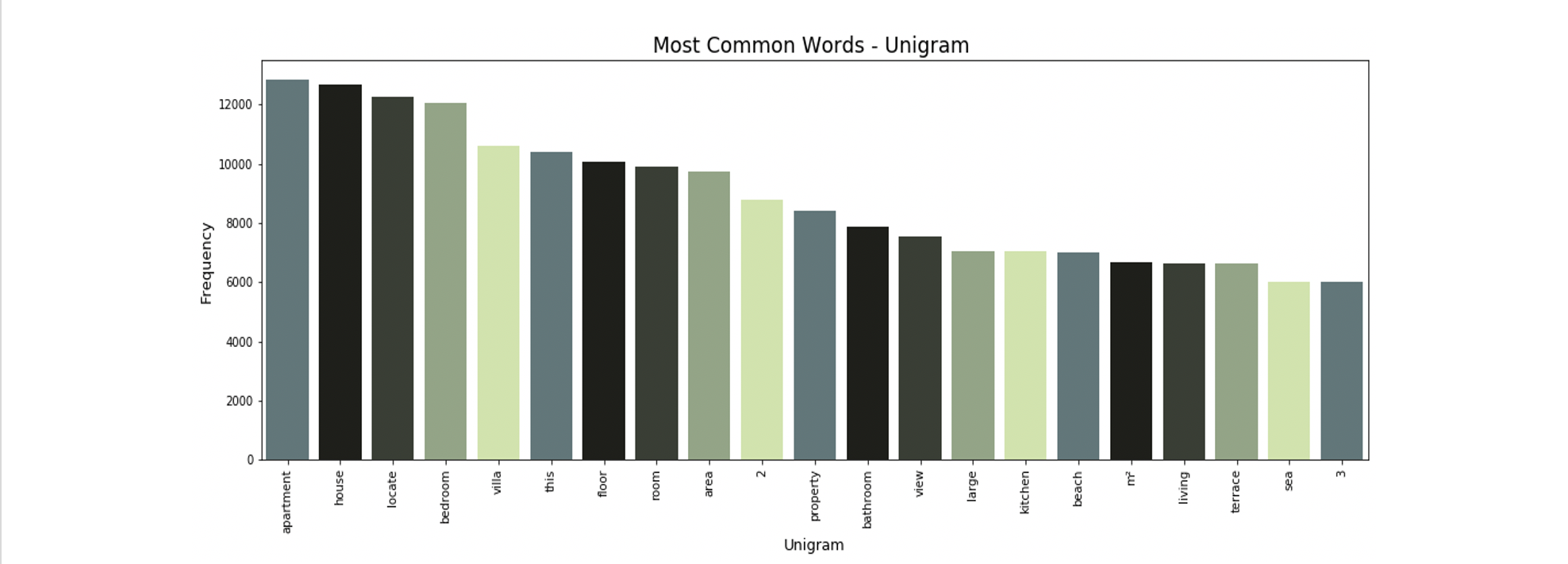
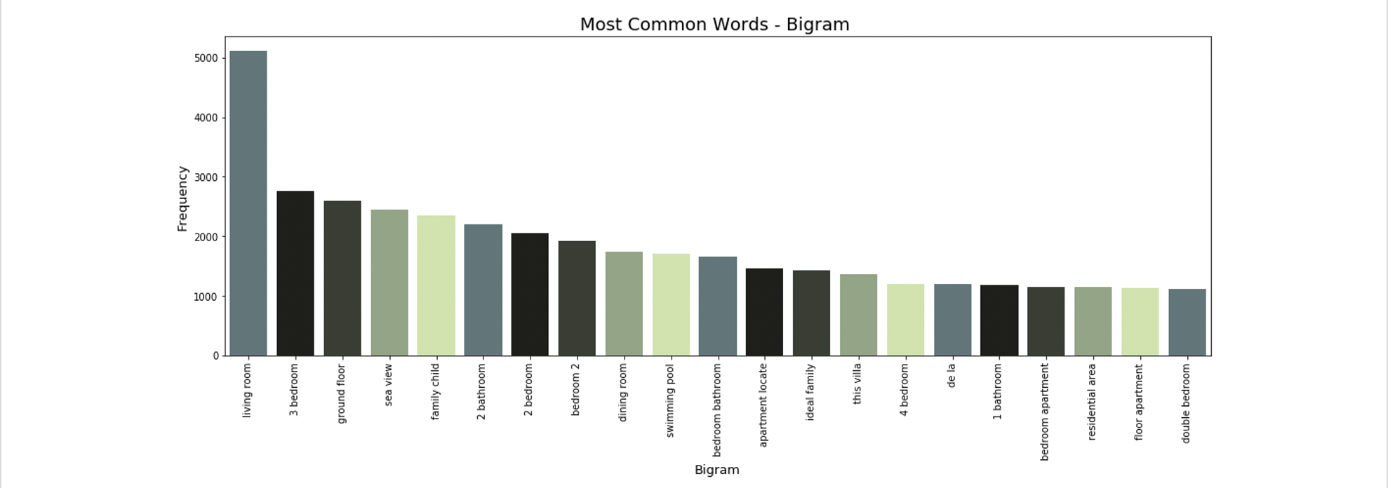
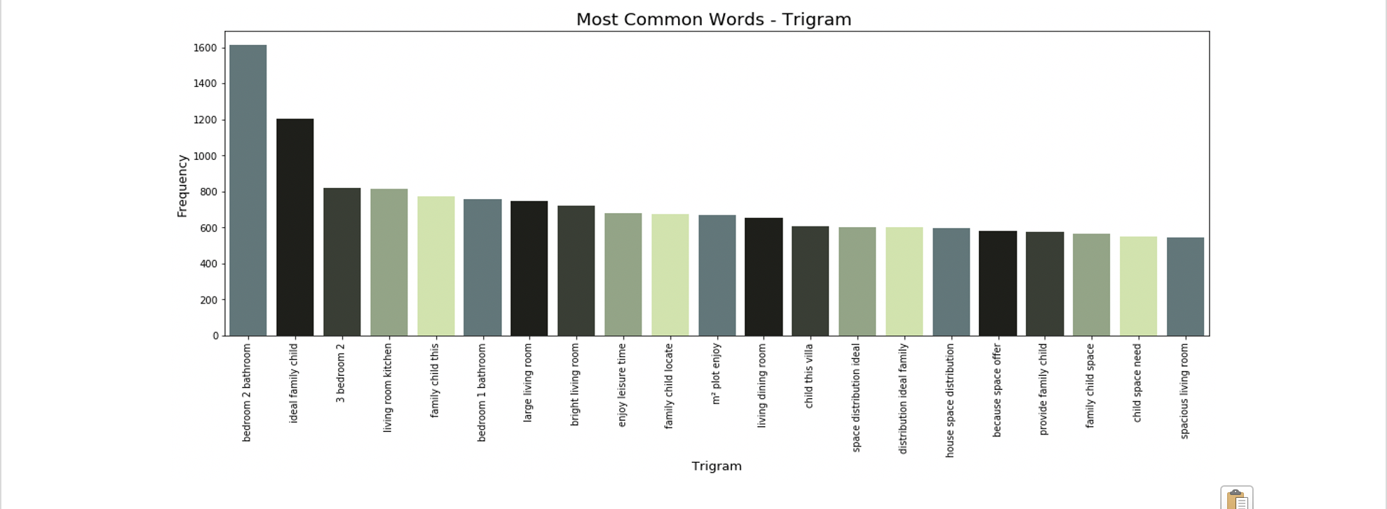
The most common uni-, bi- and tri-grams are “apartment”, “living room” and “bedroom 2 bathroom”. These are all typical real estate-focused words, and many of them are likely not helping our model’s prediction of price. For example, the most common trigram “bedroom 2 bathroom” is likely arriving from all X bedroom 2 bathroom listings. This information is already captured by our explicit bedroom and bathroom features, so it’s not giving our model any new information and should be excluded.
Other terms like “living room” should also be excluded- it’s likely that virtually all homes listed have a living room, and it’s unlikely that the inclusion of this word in a listing has much impact on the target variable of price.
05 Repeat
After looking at our initial visualisations, we decided to add the following steps in our text pre-processing pipeline:
01 Removing additional real estate-specific stop words, like those listed here:
real_estate_stopwords = [
    "area",
    "province",
    "location",
    "plot",
    "hectare",
    "m²",
    "m2",
    "sq",
    "sale",
    "square",
    "meter",
    "bedroom",
    "bathroom",
    "room",
    "living",
    "kitchen",
    "hallway",
    "corridor",
    "dining",
    "pool",
    "apartment",
    "flat"
    ]
For words like “bathroom” and “pool”, it was easy to justify their removal with the argument that they’re already explicitly included in the numeric features. However, with other words like “apartment”, “flat”, and “house”, it wasn’t so easy to know if we should remove them. It’s easy to imagine that whether the property is a flat or a house could have an impact on the price.
02 Remove all numeric tokens
We removed numeric tokens to avoid adding redundant information, and to assure we weren’t accidentally including our dependent variable (price) in our features.
After adding these steps to our pre-processing pipeline, the n-grams became much more interesting:
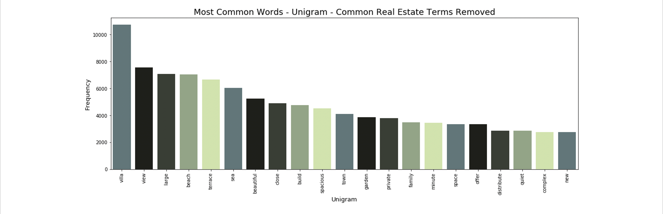
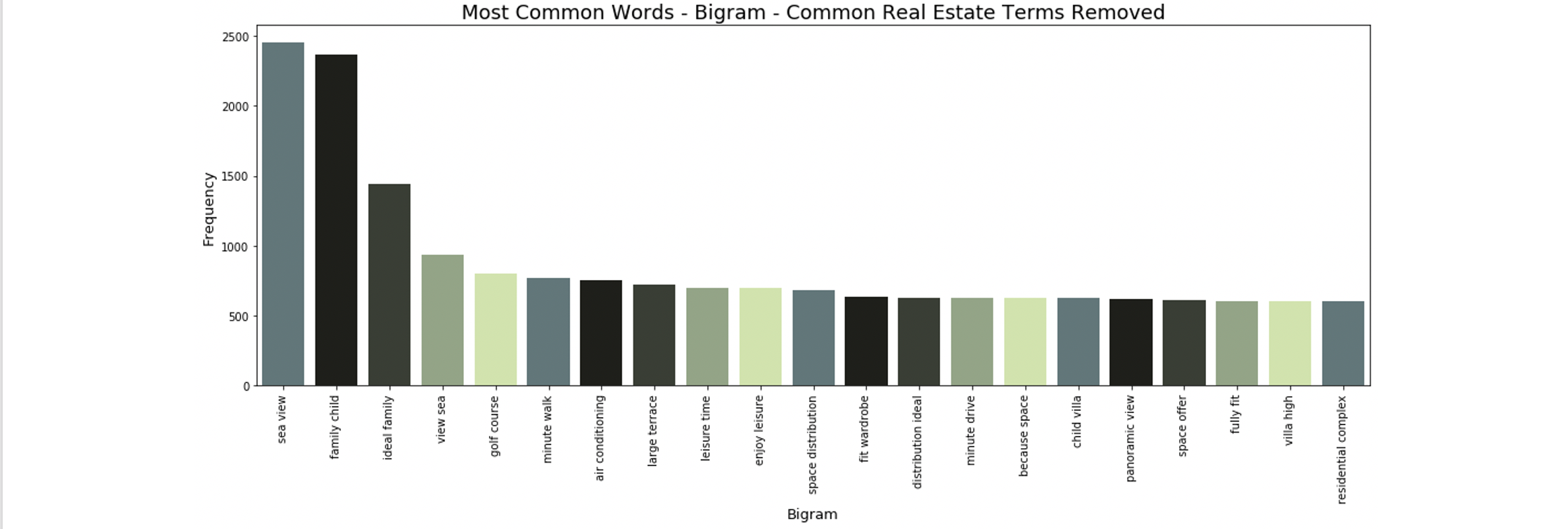
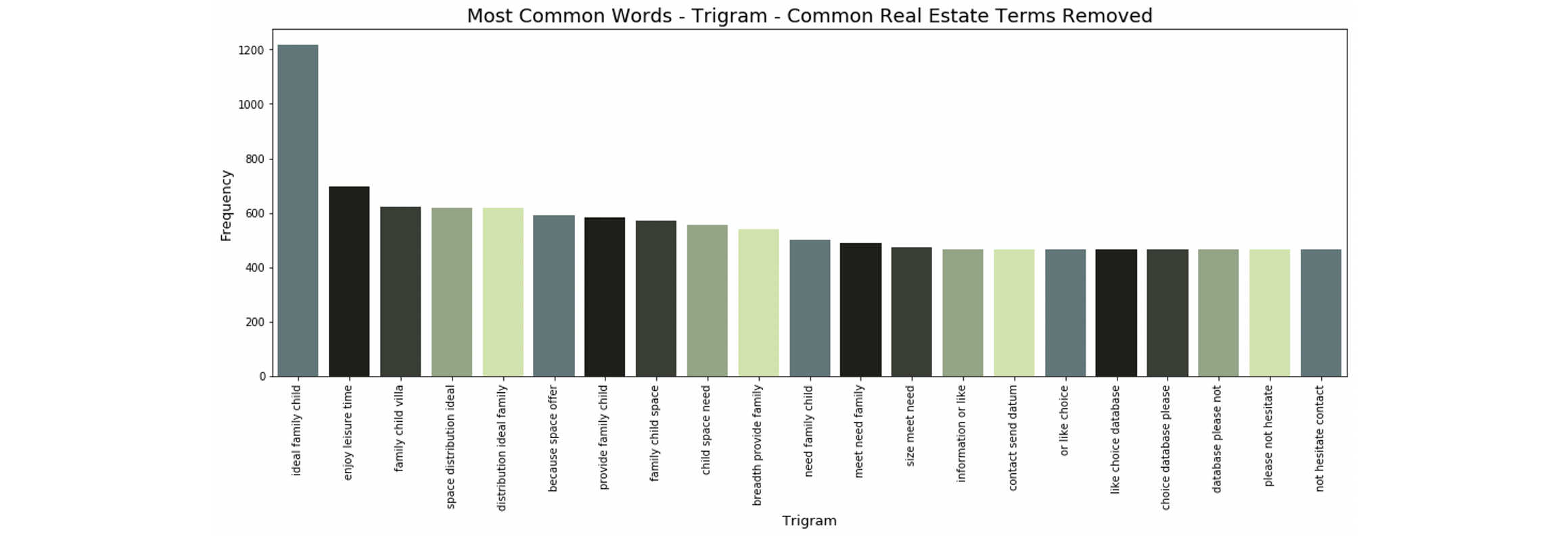
The bigrams and trigrams are no longer dominated by words like bedroom and bathroom. They now contain price-relevant terms like “sea view”, “enjoy leisure time”, and “golf course”.
Further Visualizations: Word Clouds
Word clouds are a great way to further understand text data. Our next step was to use word clouds to visualize two subsets of our corpus: the most and least expensive 5% of all observations. Our hypothesis is that the words included in these word clouds should be different: words used to describe inexpensive houses might include things like “fixer-upper” or “cozy”, whereas we might expect to see words like “dream home” or “extravagent” used to describe the most expensive homes.
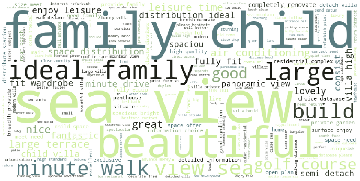
We started by visualizing the word cloud for the entire corpus of text. This is the same data used to create the n-gram visuals above.
Next we created a wordcloud for the cheapest 5% of listings, which worked out to be listings under €75,000. Since our dataset contains about 32,000 listings, the top and bottom 5% each contain roughly 1,570 listings.
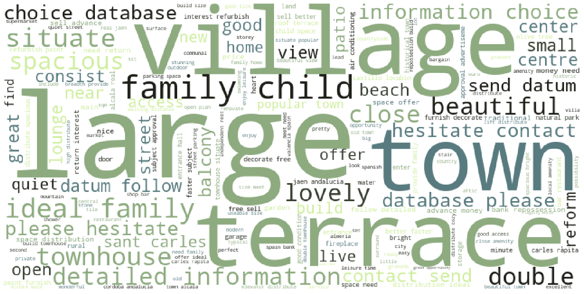
The words “villiage” and “town” appear much more commonly in the inexpensive houses- which makes sense as real estate in rural areas generally costs less than in cities. There are also many words about contacting the real estate agent or requesting information. This could signal that these cheaper homes are priced to move and the seller and real estate agent are motivated to sell.
For the word cloud of the most expensive 5% of properties, the cutoff price was €1.7 million.
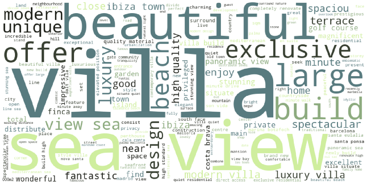
Here we can clearly see a stark difference in the most common words. Sea views are more common, as are adjectives like “luxury”, “exclusive” and “high quality”.
Now that we have our text prepared and are confident that there is a difference in the description tokens of inexpensive and expensive properties, we can turn to applying our text data to the model in the form of a TF-IDF feature vector.