Predicting Real Estate Prices

Machine Learning for predicting Spanish real estate prices.

This post is discusses machine learning model selection and performance assessment for prediction Spanish real estate prices. More specifically, in this post we compare different models based on their prediction performance on our real estate data. This post also elaborates on the workings of the Gradient Boosting model.

This post then concludes with an explanation of the best model’s performance, and the hyperparameters that led to the best model.

This post proceeds as follows:

1. Feature Pre-Processing
2. Model selection and specification
3. Model Results
4. Conclusion

01 Feature Pre-Processing

Before proceeding with any kind of prediction model, it is important to spend some time with pre-processing the features. This helps the model get as much information as possible from the data. In earlier posts we explored and explained all of our basic features and more advanced features.

While extracting these features, we saw that there were quite a few outliers which could be potentially problematic for the model. This is important to note because the decision tree models used here, in contrast to what is commonly believed, are not immune to the effects of outliers. After thorough inspection of the data and exclusion of the observations deemed outliers, the number of observations was reduced from 40,733 to 40,243 - a drop of roughly 500 observations.

The features used for training these prediction models are the following:

• No. of Bedrooms
• No. of Bathrooms
• Dummy variable for whether property has a pool
• No. of Square Meters
• Longitude of the City
• Latitude of the City
• Cluster Grouping variable
• How many Metropolis cities within 30km radius
• How many Large cities within 30km radius
• How many Medium cities within 30km radius -Dummy for whether cities is listed as “quality” city from a leading tourist website
• How far away a city with more than 100k habitats is (in km)
• Average temperature over the last 30 years
• Average total precipitation over the last 30 years
• Average wind speed over the last 30 years
• Average air pressure of the last 30 years In order to get a feeling for these variables, we take a deeper look into the continuous variables of the features listed above.

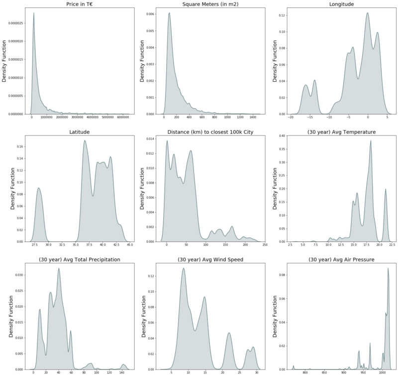
Looking at the plots, we see that many of them (especially the dependent variable: Price) exhibits a large amount of skewness. In order to work around this unfavorable distribution, we apply logs on all continuous variables. The goal of using logs is to “squish” more extreme values closer to the rest of the data. This step within the pre-processing is favored by nearly all statistical model in case of very high or low skewness.

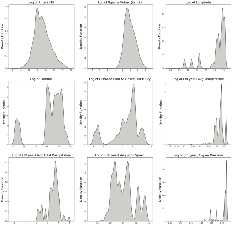
The figure below shows nicely the effect of the natural logarithm. Especially the Price variable (which exhibited the most extreme skewness before) shows a significantly improved shape. Other variables like the average air pressure may still show a skewed distribution, but the relative difference in the more extreme values is not as daunting as before applying logs.

For the upcoming prediction models, we are proceeding with the log version of the continuous variables.

02 Model selection and specification

For the task of predicting real estate prices, we rely on tree based models. We also implemented a multiple linear regression, but only as a baseline. The main reasons for applying tree-based models for this tasks are the following:

1. Ability to capture non-linear effects. This is important since it is fair to assume that the marginal effects of another bath-/bedroom within a property are not constant. Consider, for example, the benefit to a family of going from one bedroom to two bedrooms compared with the added benefit of going from nine to ten bedrooms.
2. Ability to handle sparse data. This benefit is especially noticeable when the natural language processing features are added later on, since word-vectorization results in a sparse feature matrix.
3. Tree-based models, and especially Gradient Boosting are famous for their superior prediction power. This is nicely described and explained here.

02.1 Inner Workings of Gradient Boosting

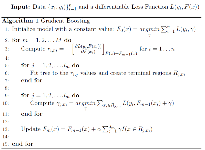
Since Gradient Boosting is our main model within this project (its superior performance is shown later), we here briefly walk through how this model works.

We begin with discussing what the Gradient Boosting model takes as an input. As with every boosting model, Gradient Boosting needs (next to data of course), a differentiable loss function. The necessity of this will be outlined later on.

Boosting is an iterative process in contrast to bagging (the category under which the Random Forest falls). That means that we start with an initial “naive” model (also called a weak learner) and then iteratively increase performance by adding further weak learners.

In the beginning, the model makes a prediction on the entire dataset. This is done by minimizing the loss function. In case of a regression problem (in contrast to a clustering problem) the loss function is most commonly the mean squared error (MSE). It is important to stress that we get only one prediction for every single observation. As expected, this first prediction will likely not do a good job. The magic happens in the next steps. In contrast to Adaptive Boosting, which in the following steps focuses on the observations the model predicted relatively badly, Gradient Boosting is rather interested in the residuals of the first step. Namely, it takes the residuals from the first step and fits a tree model on them.

The tree model algorithm then splits the residuals into different leafs. The last leaf of a tree model is called its terminal leaves. The Gradient Boosting algorithm then forms a prediction for all terminal leaves. This is done by, again, minimizing the loss function. This leaves us with a prediction of the residual (also called pseudo residuals in this application) for every terminal leaf.

The last step is to go back to our initial prediction made in the first step. This time we make a more educated guess about our prediction of the actual value. As a baseline for our new prediction we use the initial “naive” prediction we estimated at the very beginning for all observations. We then add our terminal leaf-specific residual prediction to it.

Lastly, since we do not want to overstate our result of the residual prediction we add to the baseline, we multiply that residual prediction by a factor called the learning rate. This learning rate, which is hyper-parameter we can tune, allows us to tell the model how much emphasis it should put on the residual prediction we did.

0.2.1.1 The Learning rate

When adjusting the learning rate, it is important to be aware of the trade-off that comes along with it. A learning rate that is too high leads to jumpy or scattered predictions can cause the algorithm to be unable to find the actual minimum of the loss function. On the other hand, if the learning rate is too low, the model is not adjusting enough and has a hard time to jump away from the “naive” first guess. This could lead to the model getting stuck within a local minimum and not being able to find the desired global minimum.

0.2.1.2 Number of trees

Another important hyperparameter which interacts with the learning rate is the number of trees fitted. How often the algorithm of the Gradient Boosting model should run is also a hyperparameter we can set for the model. The higher number of trees, the more time the algorithm has to improve its prediction. When the learning rate is fairly low, we need to give the model enough iterations to make improve its initial estimate. Conversely, when we set the learning rate very high, less trees are needed.

The following mathematical explanation summarizes how the Gradient Boosting model works. Here we have n observations, built M trees with J terminal leaves. Gamma denotes the prediction of the residual and F the prediction of the actual observation (not the residual). y denotes the true value of the observation. R describes the terminal region of of a tree.

02.2 Code implementation

Having understood the theory behind Gradient Boosting, we will now take a look into the implementation of the algorithm. The library used in this example is scikit-learn. As discussed above, two important hyperparameters of the boosting model are the learning rate and the number of trees (also called estimators). Since these hyperparameters are critical for the overall model performance, it is wise to test out several values for them. This is done through the GridSearchCV command shown below. The results of the GridSearchCV are elaborated on in the next section.

The differentiable loss function used is negative mean squared error, which is the most commonly used loss function for the regression application of Gradient Boosting.

def gb_score(X, y):
    # Model assignment
    model = GradientBoostingRegressor
    # Perform Grid-Search
    gsc = GridSearchCV(
        estimator=model(),
        param_grid={
            'learning_rate': [0.01, 0.1, 0.2, 0.3],
            'n_estimators': [100, 300, 500, 1000],
        },
        cv=5,
        scoring='neg_mean_squared_error',
        verbose=0,
        n_jobs=-1)
    # Finding the best parameter
    grid_result = gsc.fit(X, y)
    best_params = grid_result.best_params_
    # Random forest regressor with specification
    gb = model(learning_rate=best_params["learning_rate"],
               n_estimators=best_params["n_estimators"],
               random_state=False,
               verbose=False)
    # Apply cross validiation on the model
    gb.fit(X, y)
    score = cv_score(gb, X, y, 5)
    # Return information
    return score, best_params, gb

After finding the optimal hyperparameters using GridSearchCV, we use these hyperparameter values to initialize the final model. In order to assess model performance, and to compare different algorithms to each other, we use the fitted model in 5-fold cross validation.

Next, we take the square root of the negative values of the loss-function. This is done in order to get the so-called root mean squared error (RMSE) which is easier to interpret than the MSE, which is in squared units. The reason we take the negative of the loss function values is to remove the negative sign. This step is necessary in order to apply the square root, given that the negative mean squared error results in a negative loss.

def cv_score(model, X, y, groups):
    # Perform the cross validation
    scores = cross_val_score(model, X, y,
                             cv=groups,
                             scoring='neg_mean_squared_error')
    # Taking the expe
    # of the numbers we are getting
    corrected_score = [np.sqrt(-x) for x in scores]
    return corrected_score

02.3 Hyperparameter tuning

As mentioned in the prior section, hyperparameter tuning represents an essential part of the model choosing process. For this process GridSearchCV is applied, which tries several values for each pre-defined hyperparameter. This is done through Cross-Validation in order to prevent overfitting. The table below shows which hyper-parameters are chosen to be tested and which values ended up chosen, given superior model performance.

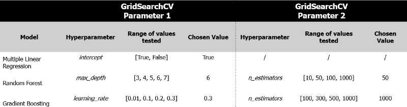
As seen above, Multiple Linear Regression only tests whether to use an intercept. This is done because there are simply no other hyper-parameters to tune for this model.

The Random Forest ends up choosing relatively few (50), but deep (depth of 6) trees. Especially the number of trees is in stark contrast to the number of trees chosen by the Gradient Boosting model, which chose 1,000 trees. Next to that, we also find the learning rate to be relatively high, with a value of 0.3.

It has to be said that performance of Gradient Boosting machines are generally worse for smaller learning rates. Furthermore, fitting more trees allows the model to make more granular predictions and allows the algorithm to fit the data better. Hence, even though both hyper-parameters seem large, they are likely well be justified.

03 Model results

03.1 Model selection

After all three model are initialized with the best-fitting hyper-parameters, their performance is evaluated. This is done through the Cross-Validation scoring code shown in section 02.1.

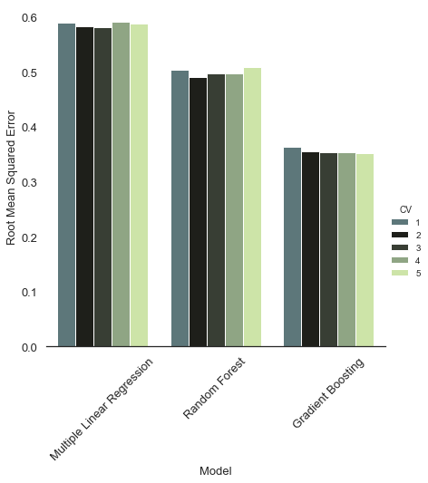
It is clearly visible that the benchmark of the Multiple Linear Regression performed the worst across of all 5 validation sets. The Random Forest performs better than the benchmark, but still nowhere close to the performance of the Gradient Boosting algorithm. Given the out-performance of the Gradient Boosting model, we will continue our analysis with the hyperparameter-tuned Gradient Boosting model.

03.2 Feature Importance

The Gradient Boosting model is next applied to the test data, which was separated at the beginning of the model selection through the following code:

X_train, X_test, y_train, y_test = train_test_split(final_x, y,
                                                    test_size=0.2,
                                                    random_state=28)

We set a random state and kept it the same for reproducability across different models. Now let’s take a look at the variable importance to assess which of the created features were most helpful to the model in predicting Real Estate price.

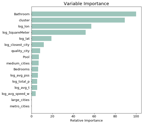
From the chart above we can see that the most important variables are those which came already with the scraping - namely the basic features of how many bathrooms the estate has and how many square meters. Furthermore, the location (longitude and latitude information) of the city of the location also plays an important role in explaining the price.

Interestingly, the cluster variable turns out to be the second most important variable. This confirms our initial belief that condensing the information of several variables to one number in the form of a cluster gives the model an easier time in allocating a property to its correct price group.

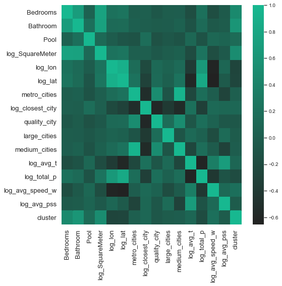
The results of the variable importance chart above should be interpreted carefully. The finding that the number of bathrooms turns out to be so much more important than the number of bedrooms, for example, could be simply explainable by the fact that these two variables are highly correlated with one another. In this case, the model is not able to separate the explanatory power of the two variables. Looking at the correlation matrix below, our believe of the positive correlation between number of bedrooms and bathrooms is confirmed - they have a correlation of 0.8.

It is important to remember that our goal was never to pin down the causal effect of propery prices, but to build a model which results in a low prediction error. The difference between these two goals is important. When interested in quantifying the effect of certain features on the dependent variable (e.g. important in policy making), it is essential to also assess the multicollinearity of the independent variables. Given our more straightforward task of building a low prediction error model the econometrical correctness of our features, is of lesser importance.

03.3 Model Assessment for Price Quintiles

Since the dependent variable in our model (Price of the property) was log-transformed in the beginning for better distributional behavior, we have to take the exponential of the predicted log-price values. Afterwards we use the mean absolute percentage error (MAPE) in order to assess the model’s performance. The reason for choosing the MAPE is the large absolute value difference between the price quintiles. For example, if our MAE (Mean Absolute Error) was €100,000, this would be over 100% MAPE for a house costing €50,000, but only a 10% MAPE for houses costing €1 million.

# Getting the predictions
gb_predictions = gb_model.predict(X_test)
# Bringing them back to normal scale and calculation of MAPE
scale_pred = np.exp(gb_predictions)
scale_y = np.exp(y_test)
mape = (abs(scale_pred - scale_y)/scale_y) * 100

In order to see whether the model predicted low- and high-priced houses equally well, we split the predicted data into ten price buckets, using the actual price of the property. That means that we calculate separate MAPEs for each price quintile.

The graph below offers us interesting insights into the model performance. Namely, it shows that the model performance is relatively consistent for all price quintiles except the for the first quintile. This quintile contains the least expensive ten percent of houses.

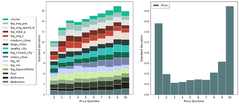
One potential reason that the model under-performs on the inexpensive houses could be the amount of variation of the features within the different price quintiles. The chart below tries to shed some more light on this. The graph on the left shows the accumulated standard deviation of all 16 features of the model. The right side shows the variation of the dependent variable, namely the log-price.

The graph shows nicely one potential reason for the struggle of the model to explain the price variation for the cheapest quintile. Namely, the amount of variation is the lowest, as visible in the right graph. Additional to that, we find that the amount of variation in the dependent variable for that price group is relatively high. This combination is dooming for any prediction model, facing a high amount of variation in the variable it wants to explain, but nothing to explain it with.

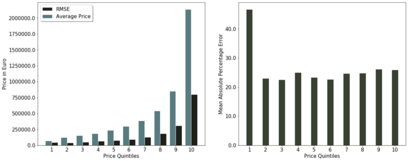
One might rightly ask why we chose MAPE as an accuracy assessment. An alternative could be, for example the root mean squared error (RMSE). The graph below sheds some light why the MAPE seems like the better fit.

On the left side of the chart below, we see that the RMSE of the lowest price group might seem superior when compared to the RMSE of higher price groups. That superior performance disappears when considering the average price of the quintile.

The reason for the weakness of RMSE as a performance assessment for this prediction task is its absolute nature. For property prices, it makes a difference whether the predicted price is off by €50,000 when the property costs multiple million or only €100,000.

Given that we are more interested in the relative error and not in the absolute one, the mean absolute percentage error seems like the superior accuracy assessment.

04 Conclusion

In the next post we show several examples where the model under-performs and explain why that is the case. Furthermore, we apply natural language processing to use text features next to the quantitative features to explain the price of properties.