
Using the power of transfer learning for building a flower classifier
In this blog-post we discuss the concept of transfer-learning and show an implementation in Python, using tensorflow. Namely, we are using the pre-trained model MobileNetV2 and apply it on the Oxford Flower 102 dataset, in order to build a flower classification model. Lastly, we deploy the trained model on an ios device to make live predictions, using the phone’s camera. The Github Repository for this project can be found here.
The concept of Transfer-Learning
The concept of transfer-learning is best understood when applied to real-life examples. If, for example, a person has played the piano for many years, this person will have an easier time picking up guitar, compared to a person who never played any musical instrument before.
That does not imply, of course, that the person who has prior piano experience is going to be perfect at playing the guitar right away, but the yearlong finger practice of playing piano and the development of having a good ear in music, makes it easier for that person to learn.
It is important to note that this synergy effect were only possible because playing piano and playing the guitar are somewhat related. If the person who played piano for many years is now trying to learn to play American Football, it is less likely that this person will have an advantage. Hence, whether the previous training of concept A is beneficial for concept B depends on whether concept A and B bear any similarities to one another.
The very same idea applies to transfer-learning. Let us assume that we have a model which is very strong in detecting whether an apple is portrayed in a given image. Chances are good that we could use this model to detect pears as well, since pears and apples are similar (both round fruits). It will definitely not be as strong as a model that was trained entirely on pears, but in situation where we do not have that many trainings images of pears, it is better than nothing.
That the apple detection would work also on detecting pears is only because apples and pears bear some common characteristics, like for example color and shape. If we would, on the other hand, take the apple detection model and try to detect cars with it, we will likely have terrible performance.
The question might arise why we are not simply building one model for each job: one model for detecting apples, one model for detecting pears, and so on. The reasons why this is sometimes not feasible are multi-fold. It could be, for example, that we lack the computational power, the time, or even the amount of images needed to train a classification model that performs well. Especially the latter reason is a common problem within image detection.
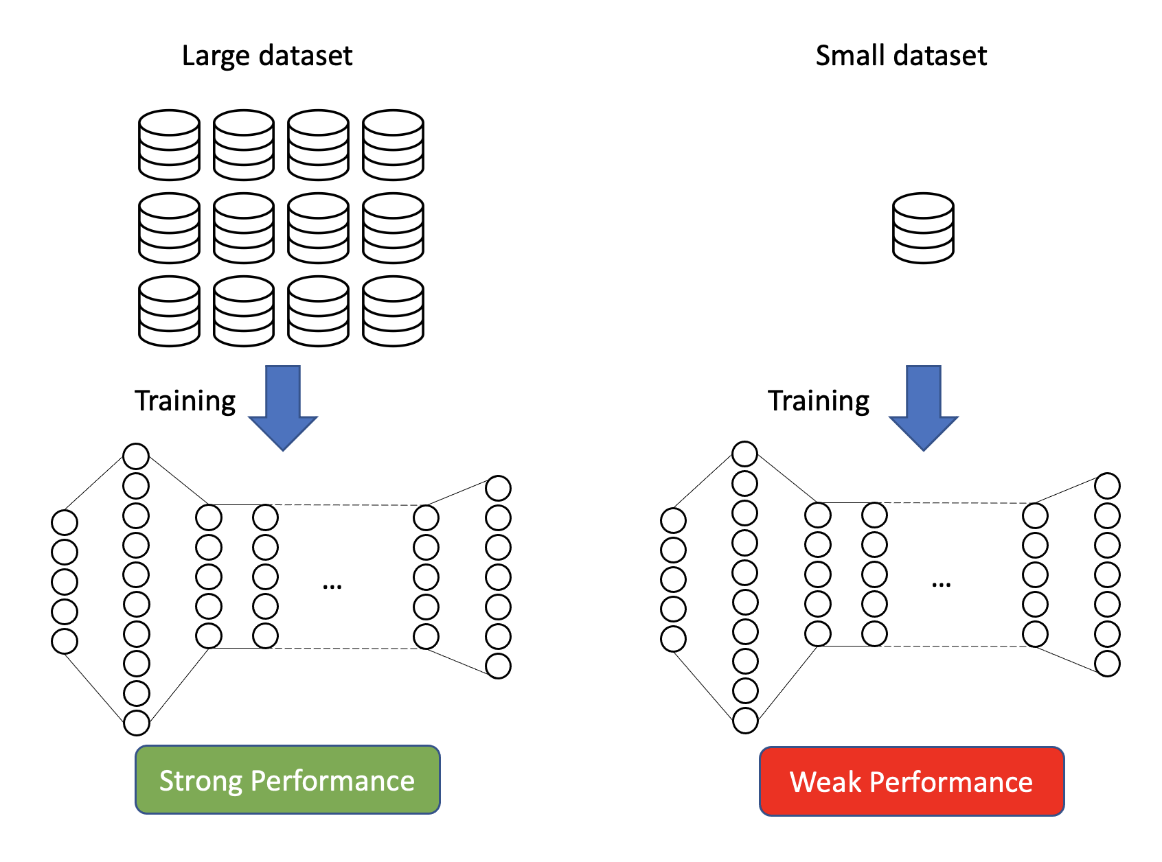
The reason why a small amount of images leads to a poor performing model is easily understood when considering the workings of a neural network. When initializing a neural network, all weight parameters are initialized randomly. Through the training process these weight parameters are constantly adjusted, using back-propagation based on gradient descent. If we do not have enough images of the object we would like to classify, the network is not going to have a sufficient amount of data in order to adjust the weights appropriately (i.e., learn).
Transfer-learning can help in those situations. That is because of the workings of convolutional neural networks (CNNs), which are the gold standard when working with image data. While many details of CNNs are not fully explored, it is established that especially the lower levels of those models learn general shapes and patterns of the images. In the final layers of the networks all these shapes and patterns are put together to make up for the final object.
When using a pre-trained model on a different domain than it was originally trained for, we cannot make use of the top-layers of the pre-trained model since they are too specific to the initial use-case. The lower-levels of the network, on the other hand, come in very handy since detecting shapes and patterns is an essential part of image recognition, as is going to be needed for the new domain as well.
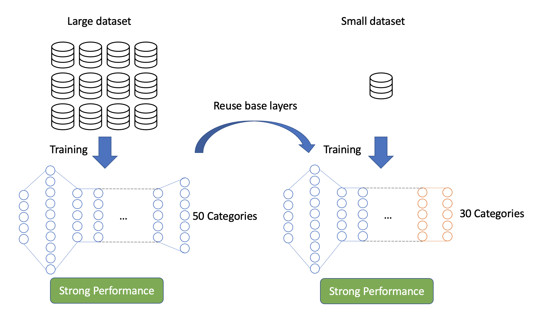
Therefore, we simply separate the pre-trained model into two pieces. The first piece, the layers below the very top are referred to as the base-model. The job of these layers is to detect shapes and patterns and also to combine those. The second piece are the top-layers. These layers are specific to the objects the model is classifying. This second piece is unwanted when changing the domain the model is supposed to classify, and therefore simply removed.
After removing the top-layer from the base-model, we simply stack one or several untrained layers on top of the headless base-model. It is important to note that the new top-layers can also have a different amount of categories compared to the previous top-layers. That means, if the pre-trained model was originally trained to classify 50 different dog breeds, we can remove the last dense layer which outputs a vector with length 50, and add a layer with 30 categories, in order to classify 30 different cat breeds.
When stacking one or more top-layers on top of the lower levels, we have to re-train the entire model. It is important to note that we are solely intending to train the top-layers, not the base-model. We achieve that by freezing the weights of the base-model and therefore only training the newly added top layer with image data from the new domain. That is because jointly training the pre-trained model with the randomly initialized top-layers would result in gradient updates that are too large, and the pre-trained model would forget what it originally learned.
Through that approach the model is much faster in correctly classifying the objects from the new domain, since it does not spend time with learning how to detect shapes and patterns, but solely on how to identify what the combination of such shapes and patterns represent.
After training the top-layers we then can go one step further and train the entire model a bit more, by unfreezing some top-layers of the base-model and re-training those as well. It is crucial at this point to use a smaller learning rate, in order to not cause large gradient updates which would shake the foundation of the model.
MobileNet V2
After covering the general idea of transfer-learning, we are now moving in the direction of implementing our own transfer-learning model. For that we first have to find a solid pre-trained model. As explained above, it is important for the cross-learning effects to happen that the pre-trained model is generalizable. Therefore, most of these pre-trained models are initially trained on very large image datasets with hundreds of categories. For that reason, many of the pre-trained models are trained using the ImageNet database. This database offers 1000 categories and over one million training images.
When choosing which pre-trained model to go for, we were influenced in our decision by the fact that we are interested in deploying our final model on a mobile device. This causes obvious limitations in storage space, processing speed and energy usage, due to the decreased capactities of mobile phones. Lucky for us, there is a pre-trained model for exactly that purpose, namely the MobileNet V2, which was developed by Google.
Model architecture
Before implementing that model right away, we take a look at its workings and what makes the model the better choice for being deployed on a mobile phone in contrast to any other model. For that we take a look at the original paper. More specifically, the model architecture of the network. The graphic below shows the different layers which were used when initially training this model. Each line represents one layer, which is repeated n times.
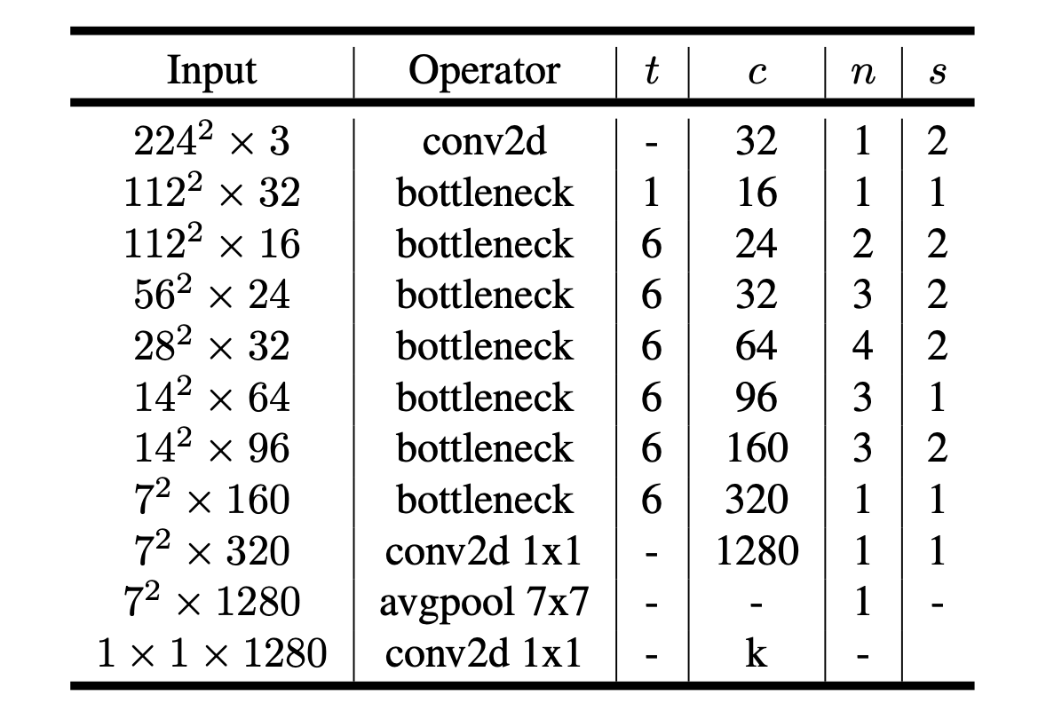
The MobileNetV2 starts with a traditional convolution before starting to apply the so-called bottleneck operator. This operator is elaborated on in more detail in the following sections. The main idea of these bottleneck layers is that they try to maintain the same level of accuracy as original convolutional networks, while being computationally cheaper. The size of the feature maps being passed from one layer to the next, are denoted by the variable c, while the stride parameter is denoted as s. The parameter t describes the expansion factor, which is the amount by which the number of channels are expanded within the bottleneck methodology.
As with most image classification models we notice how the number of channels gradually increases, while the image size decreases before collapsing the image into a 1x1 with k channels using average pooling and again a traditional convolution.
Bottleneck Sequence
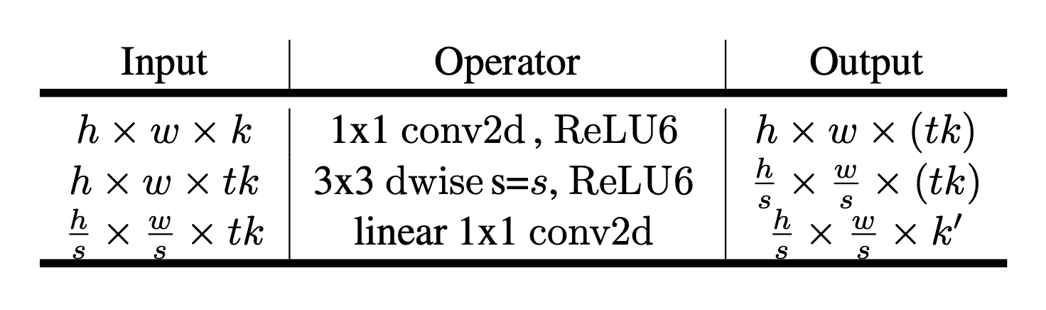
The main difference between the workings of the MobileNetV2 and other image classification model architectures are the usage of these so-called bottlenecks. The original paper describes bottlenecks as a sequence of three things - expansion layers, a depth wise convolution, and a projection layer. The following table, which was extracted from the original paper, nicely shows how the input and output sizes change when applying the bottleneck sequence.
One noteworthy aspect we gain from the table is that this approach is not using any pooling mechanism, and is altering the image’s height and width solely using the stride parameter.
Expansion Layer
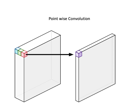
As the name suggests, what the expansion layer does is that it increases the number of feature maps of the output. This is done by applying multiple 1x1 kernels on the image and through that, increasing the size of the channels without altering the height or width of the image. This can also be seen from the table above. The original paper describes this process as a form of unzipping the image into a larger workbench. By how much we are increasing the number feature maps is a user defined input defined as t. The original paper set the default value equal to six.
Depth wise convolution
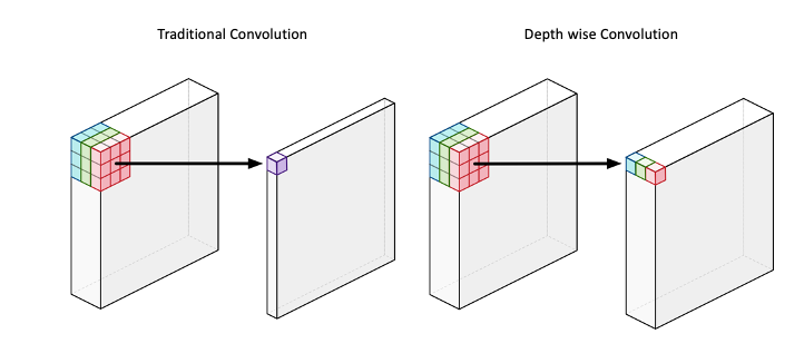
After increasing the number of channels through the expansion layer, we then apply a so-called depth-wise convolution. Depth wise convolution is very similar to traditional convolution, with the only difference being that the result is not one pixel within a feature map, but multiple.
To better understand that, we quickly explain the workings of traditional convolution. Traditional convolution applies one (usually) squared kernel to an image, which then calculates the dot product with every feature map respectively and then calculates a weighted sum of all dot product results in return one single number. The resulting number of feature maps when applying a kernel to an image is equal to one.
When applying depth wise convolution, we still apply the kernel to the image and calculate the dot product for every feature map. The difference is that we are then not summing the results of all feature maps together, but rather only sum the dot products for each feature map individually. This approach results in us having the same amount of feature maps before and after applying the convolution. This is also visible by looking at the second row of the table above, in which it says that both the input and output are equal to $tk$.
Projection layer
Lastly, we apply a so-called projection layer. What this layer is doing is that it shrinks the number of feature maps. This is done by simply using again a 1x1 kernel, but this time not in order to increase the number of feature maps, but rather in order to decrease them. The amount by which the projection layer shrinks the number of feature maps is a user-defined input, denoted as c.
Graphical Example
To better understanding the combined workings of the bottleneck sequence, we will take a look at an example. Let us assume that we have an image with the sizes 128x128x16. When applying the expansion layer we increase the number of feature maps of the image. Using the default expansion factor of six, the number of channels increases to $16*6=96$, while not changing the width or height of the image.
The second step would then be to apply the depth wise convolution. Given that the depth wise convolution does not change the number of channels, we do not have any change in the number of feature maps. Assuming a stride equal to 1, we also do not change the number of height or width.
Lastly, we decrease the number of feature channels again, using the projection layer. Herein we set the number of desired output channels equal to 24, which is therefore going to be the resulting number of output channels.

Motivation
The question might be asked why we are doing all of this instead of simply using traditional convolution. The reason for this is mainly already answered by the invention of MobileNetV1. In contrast to MobileNetV2, V1 consists only of the depth wise convolution plus the projection layer. This combination is by the original paper referred to as Depth wise separable convolution.
In order to gain a more mathematical understanding of why the depth wise separable convolution is computationally beneficial is found when considering the number of computations both methods have to go through. Traditional convolutions have a computational cost of:
\[D_K \cdot D_K \cdot M \cdot N \cdot D_F \cdot D_F\] \[\begin{align} D_K &= \textrm{Kernel size} \\ M &= \textrm{Number of input channels} \\ N &= \textrm{Number of output channels} \\ D_F &= \textrm{Feature map size} \\ \end{align}\]In contrast to traditional convolution, depth wise convolution does not take the number of output channels into consideration, since it creates as many output channels as it has input channels by definition. Adjusting the number of output channels is then conducted by the projection layer. Both costs are then in the end summed together, resulting in the computational cost of the depth wise separable convolution:
\[D_K \cdot D_K \cdot M \cdot D_F \cdot D_F + M \cdot N \cdot D_F \cdot D_F\] \[\begin{align} D_K &= \textrm{Kernel size} \\ M &= \textrm{Number of input channels} \\ N &= \textrm{Number of output channels} \\ D_F &= \textrm{Feature map size} \\ \end{align}\]When then calculating how many times the depth wise separable convolution is superior to the traditional convolution, we find the following:
\[\frac{D_K \cdot D_K \cdot M \cdot D_F \cdot D_F + M \cdot N \cdot D_F \cdot D_F}{D_K \cdot D_K \cdot M \cdot N \cdot D_F \cdot D_F} = \frac{1}{N} + \frac{1}{D^2_K}\] \[\begin{align} D_K &= \textrm{Kernel size} \\ M &= \textrm{Number of input channels} \\ N &= \textrm{Number of output channels} \\ D_F &= \textrm{Feature map size} \\ \end{align}\]Assuming a Kernel size of 3, we then find that the convolution method of MobileNet is 8 to 9 times more efficient compared to traditional convolution.
The computation gains are the main motivation of using MobileNet overall. The difference between V2 and V1 are mostly the idea of zipping and unzipping the image within each bottleneck sequence, which further reduces the computational costs.
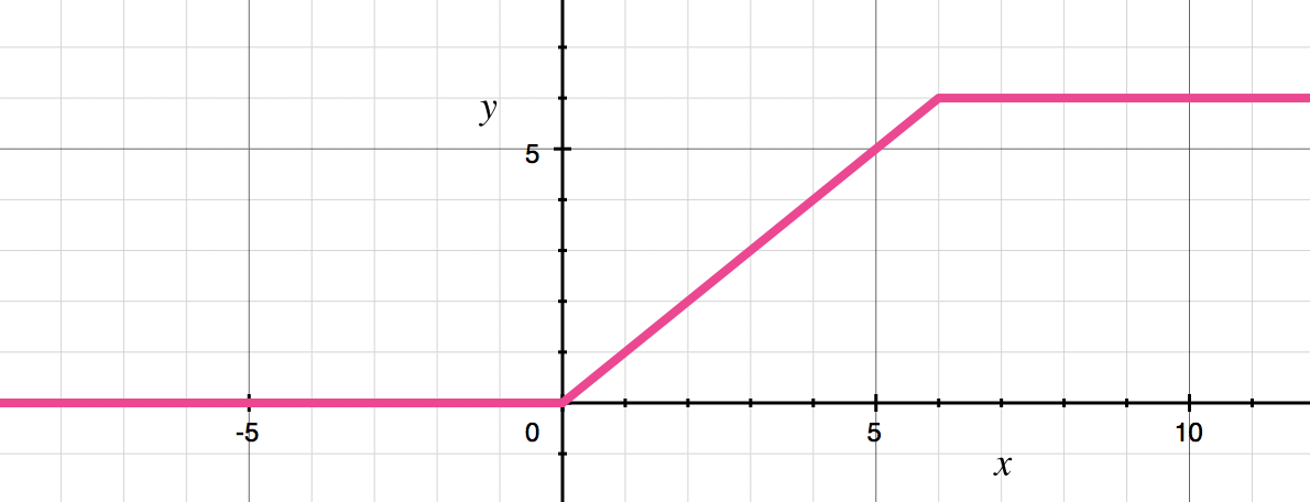
Side note: ReLU6
It is also interesting to note that the MobileNetV2 does not use a traditional ReLU function, but rather a so-called ReLU6 activation function. As the name probably already suggests, this caps all positive values at positive six, preventing the activations from becoming too large.
Oxford Flower 102
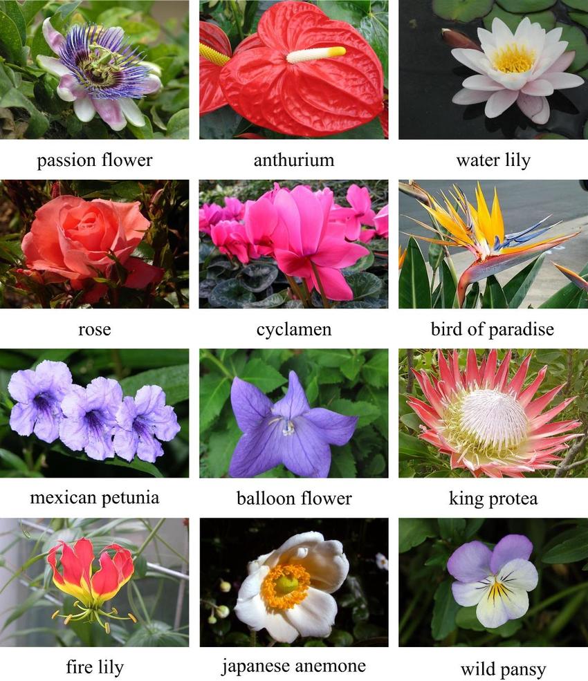
In order to show the power of transfer-learning we chose the Oxford Flower 102 dataset, which can be found here. This dataset contains, as the name suggests, 102 different categories of flowers in the United Kingdom. Each flower category contains between 40 and 258 images, respectively. Obviously, this amount of data is far too little to train a sophisticated neural network from, which makes it a good testing example of transfer-learning.
Code implementation
The implementation of this transfer learning example was done in tensorflow. Choosing tensorflow over PyTorch did not have any particular reason, as both frameworks have a significant amount of content about transfer-learning. The repository for this project is found here. The final implementation of the trained model into an ios application is conducted following the tutorial from tensorflow’s repository.
Data Structure
In contrast to many other blog-posts which try to show intuitive output after every code cell, this post works a bit differently given the packaged code. Instead, this post shows all classes used in building the model individually and elaborates on its workings.
In order to have a better understanding of how the different classes interact with each other, we start by showing the src folder for this project.
import seedir as sd
sd.seedir("../src", style="lines", exclude_folders="__pycache__")
src/
├─config.json
├─data_loader.py
├─utils/
│ ├─config.py
│ └─args.py
├─coreml_converter.py
├─model.py
├─trainer.py
└─main.py
As usually done, all major classes are constructed in their own file and then called and executed within main.py . All kinds of hyper-parameters for every class are stated within the config.json file and called by using an argparser function defined in the folder utils.
Data Loader
The first step we have to do after downloading the images is to load them into Python. This step was less straight-forward than originally thought. This is because the Oxford Flower dataset has the interesting property of having substantially more test data than training data. This might be an interesting challenge for many, but for our use-case, in which we would like to end up building a strong classification model, we would rather have more trainings data.
In order to self-set the train to test data ratio, we have to unpack all images and shuffle them ourselves. These steps are outlined in the methods _loading_images_array and _load_labels . Since labels and images are stored within two separate files, we have to make sure to correctly align and match image and label. This is done by sorting the image names in ascending order before attaching the labels. The labels have to be one-hot encoded, in order to be properly used within the prediction algorithm.
We decided to use the preprocessing class ImageDataGenerator from the preprocessing package from tensorflow. Using this preprocessing method allows us to easily apply the appropriate data augmentation settings for the images. One has to be aware that when using the pre-trained model MobileNetV2, one has to apply the related pre-processing function for that very model. This is necessary since the input images have to resemble the same kind of images which were used when training the model in the first place.
Furthermore, we applied several data augmentation techniques to the training data. This is commonly done in situation in which we have only a limited amount of training data. In contrast to the training data, the validation and test data is not augmented in any way other than the necessary MobileNetV2 pre-processing. Classifying the flower category becomes a much harder challenge for the model when the image is heavily augmented. Since the validation data is not altered in any way, those examples are much easier for the model, which results in a better performance of on the validation data in contrast to the training data, a phenomena which rarely occurs.
# %% Packages

import os
import numpy as np
import tensorflow as tf
from scipy.io import loadmat
from sklearn.preprocessing import OneHotEncoder
from sklearn.model_selection import train_test_split
from tensorflow.keras.preprocessing.image import ImageDataGenerator

# %% Classes

class OxfordFlower102DataLoader:
    """
    This class loads the images and labels and embeds them into ImageDataGenerators.
    """

    def __init__(self, config):
        self.config = config
        (
            self.train_generator,
            self.val_generator,
            self.test_generator,
        ) = self.create_generators()

    def create_generators(self):
        """
        This method loads the labels and images, which are already split into train, test and validation.
        Furthermore, we add an additional step to the preprocessing function, which is required for the pre-trained
        model. Afterwards we create ImageGenerators from tensorflow for train, test and validation.
        :return: ImageDataGenerator for training, validation and testing
        """
        X_train, X_val, X_test, y_train, y_val, y_test = self._image_and_labels()
        train_augment_settings, test_augment_settings = self._add_preprocess_function()

        # Data Augmentation setup initialization
        train_data_gen = ImageDataGenerator(**train_augment_settings)
        valid_data_gen = ImageDataGenerator(**test_augment_settings)
        test_data_gen = ImageDataGenerator(**test_augment_settings)

        # Setting up the generators
        training_generator = train_data_gen.flow(
            x=X_train, y=y_train, batch_size=self.config.data_loader.batch_size
        )
        validation_generator = valid_data_gen.flow(
            x=X_val, y=y_val, batch_size=self.config.data_loader.batch_size
        )
        test_generator = test_data_gen.flow(
            x=X_test, y=y_test, batch_size=self.config.data_loader.batch_size
        )
        return training_generator, validation_generator, test_generator

    def _add_preprocess_function(self):
        """
        This function adds the pre-processing function for the MobileNet_v2 to the settings dictionary.
        The pre-processing function is needed since the base-model was trained using it.
        :return: Dictionaries with multiple items of image augmentation
        """
        train_augment_settings = self.config.data_loader.train_augmentation_settings
        test_augment_settings = self.config.data_loader.test_augmentation_settings
        train_augment_settings.update(
            {
                "preprocessing_function": tf.keras.applications.mobilenet_v2.preprocess_input
            }
        )
        test_augment_settings.update(
            {
                "preprocessing_function": tf.keras.applications.mobilenet_v2.preprocess_input
            }
        )
        return train_augment_settings, test_augment_settings

    def _image_and_labels(self):
        """
        This method loads labels and images and afterwards split them into training, validation and testing set
        :return: Trainings, Validation and Testing Images and Labels
        """
        y = self._load_labels()
        X = self._loading_images_array()
        X_train, X_test, y_train, y_test = train_test_split(
            X,
            y,
            train_size=self.config.data_loader.train_size,
            random_state=self.config.data_loader.random_state,
            shuffle=True,
            stratify=y,
        )
        X_train, X_val, y_train, y_val = train_test_split(
            X_train,
            y_train,
            train_size=self.config.data_loader.train_size,
            random_state=self.config.data_loader.random_state,
            shuffle=True,
            stratify=y_train,
        )
        return X_train, X_val, X_test, y_train, y_val, y_test

    def _load_labels(self):
        """
        Loading the matlab file and one-hot encodes them.
        :return: Numpy array of one-hot encoding labels
        """
        imagelabels_file_path = "./data/imagelabels.mat"
        image_labels = loadmat(imagelabels_file_path)["labels"][0]
        image_labels_2d = image_labels.reshape(-1, 1)

        encoder = OneHotEncoder(sparse=False)
        one_hot_labels = encoder.fit_transform(image_labels_2d)
        return one_hot_labels

    def _loading_images_array(self):
        """
        Loading the flower images and resizes them into the appropriate size. Lastly we turn the images into a numpy array
        :return: Numpy array of the images
        """
        image_path = "./data/jpg"
        image_file_names = os.listdir(image_path)
        image_file_names.sort()
        image_array_list = []
        for image_file_name in image_file_names:
            tf_image = tf.keras.preprocessing.image.load_img(
                path=f"{image_path}/{image_file_name}",
                grayscale=False,
                target_size=(
                    self.config.data_loader.target_size,
                    self.config.data_loader.target_size,
                ),
            )
            img_array = tf.keras.preprocessing.image.img_to_array(tf_image)
            image_array_list.append(img_array)
        return np.array(image_array_list)
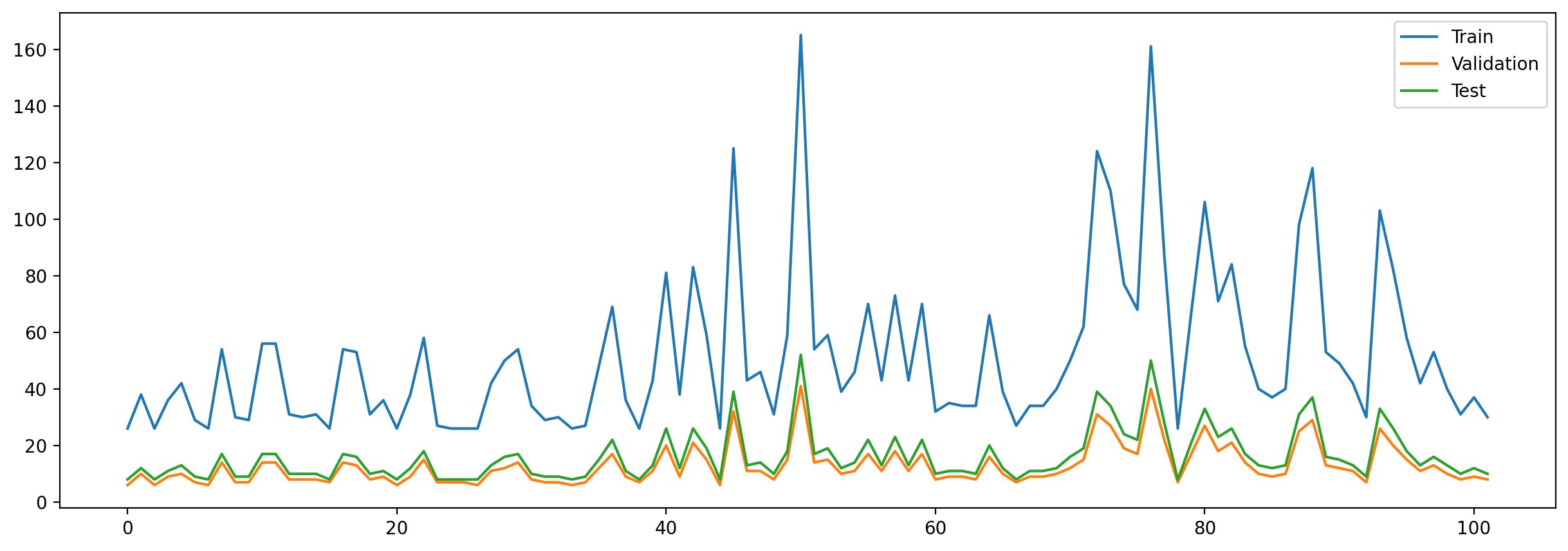
Given that we have quite a large number of flower categories to predict (102), and the fact that these categories are not balanced, we have to make sure that we have the same proportion of each class within the training, validation and test data in order to have a stronger model and a more meaningful model evaluation. This balance is ensured by using the stratify argument within the train-test split from sklearn . The following image shows the result of using that parameter: We can see that we have same proportions within the train, test and validation data.
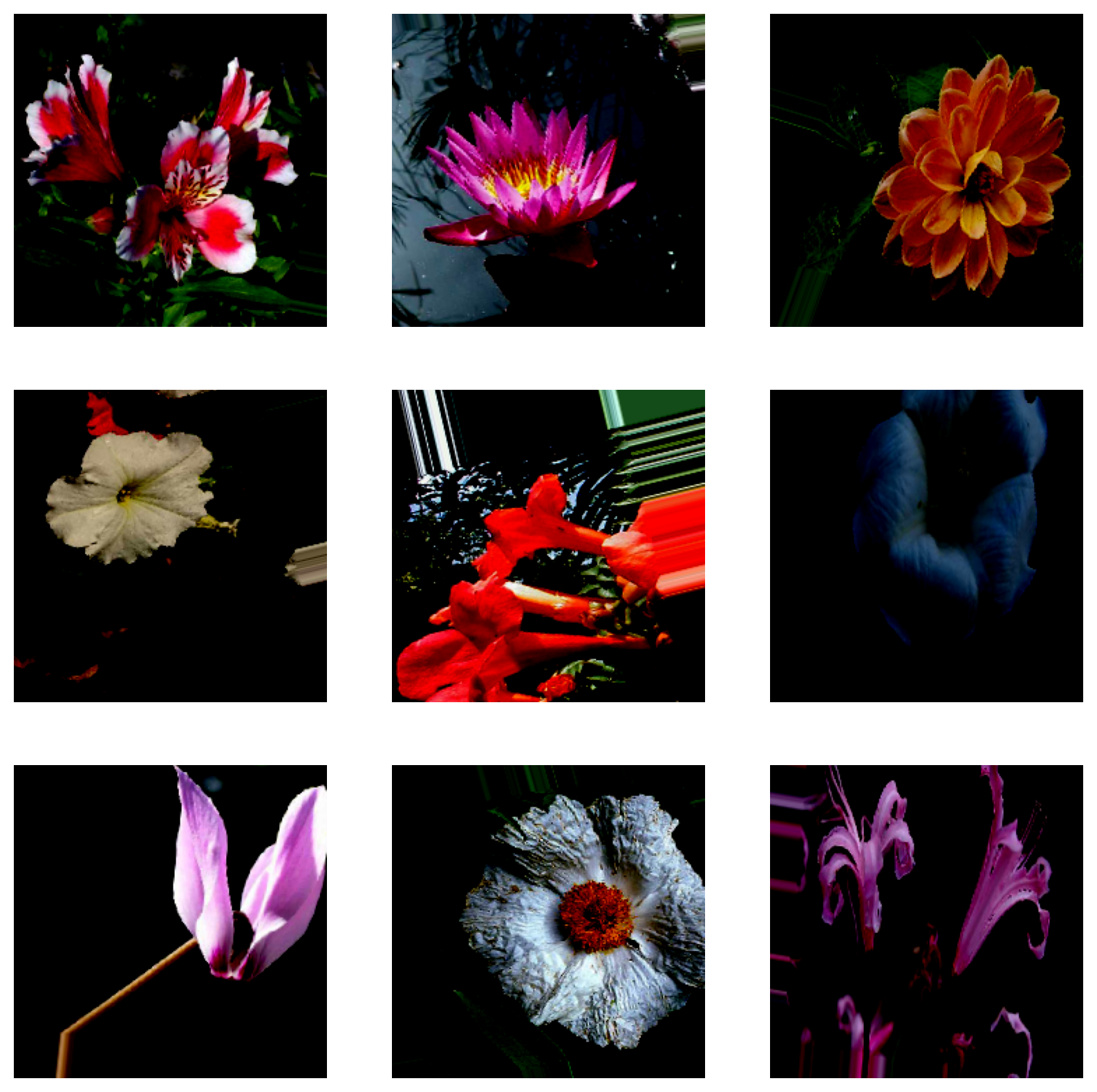
In order to also have a better understanding what the pre-processing of the images actually looks like, we show in the following nine example images from the trainings data. We see that all images are much darker than the original ones we saw before. That change of lighting comes from the MobileNetV2 pre-process function we applied. The image in the very middle of the lower matrix nicely shows the level of distortion we apply to the images. These augmentations of images are especially useful in cases like this one where we have such training little data, since it artificially increases the pool of images we can train our model with. It is to be said, though, that we are not applying these distortions on the test and validation data, since these heavy distortions don’t occur in the model’s final application and should therefore not be considered in the model’s performance on real flower-images.
Model
Now it is time to build our model. This is done in two steps. The first step loads the pre-trained model and freezes all parameters within it. We then stack a dense layer on top and solely train these weights. Furthermore, we add a dropout layer in order to prevent the overfitting of the model.
The second step, as already outlined in the explanation of transfer-learning, then describes the fine-tuning process of transfer-learning. Herein we unfreeze several of the top-layers of the pre-trained model and train them using a small learning rate in order to marginally adjust the pre-trained model in a beneficial direction.
We are using RMSprop for compiling the model, as well as a learning rate of 1e-3 for the training within the first step, and a learning rate of 1e-4 for the fine-tuning.
# %% Packages

import tensorflow as tf
from tensorflow.keras import Sequential
from tensorflow.keras.layers import Dense, Dropout
from tensorflow.keras.applications import MobileNetV2

# %% Classes


class OxfordFlower102Model:
    """
    This class is initializing the model
    """

    def __init__(self, config):
        self.config = config
        self.base_model = self.build_model()
        tf.random.set_seed(self.config.model.random_seed)

    def build_model(self):
        """
        This method build the basic model. The basic model describes the pre-trained model plus a dense layer
        on top which is individualized to the number of categories needed. The model is also compiled
        :return: A compiled tensorflow model
        """
        pre_trained_model = self.initialize_pre_trained_model()
        top_model = self.create_top_layers()

        model = Sequential()
        model.add(pre_trained_model)
        model.add(top_model)

        model.compile(
            loss=self.config.model.loss,
            metrics=[self.config.model.metrics],
            optimizer=tf.keras.optimizers.RMSprop(
                learning_rate=self.config.model.learning_rate
            ),
        )
        model.summary()
        return model

    def unfreeze_top_n_layers(self, model, ratio):
        """
        This method unfreezes a certain number of layers of the pre-trained model and combines it subsequently with the
        pre-trained top layer which was added within the 'create_top_layers' method and trained within the 'build_model'
        class
        :param model: Tensorflow model which was already fitted
        :param ratio: Float of how many layers should not be trained of the entire model
        :return: Compiled tensorflow model
        """
        base_model = model.layers[0]
        trained_top_model = model.layers[1]

        base_model.trainable = True
        number_of_all_layers = len(base_model.layers)
        non_trained_layers = int(number_of_all_layers * ratio)
        for layer in base_model.layers[:non_trained_layers]:
            layer.trainable = False

        fine_tune_model = Sequential()
        fine_tune_model.add(base_model)
        fine_tune_model.add(trained_top_model)

        adjusted_learning_rate = (
            self.config.model.learning_rate / self.config.model.learning_rate_shrinker
        )
        fine_tune_model.compile(
            loss=self.config.model.loss,
            metrics=[self.config.model.metrics],
            optimizer=tf.keras.optimizers.RMSprop(learning_rate=adjusted_learning_rate),
        )
        fine_tune_model.summary()
        return fine_tune_model

    def initialize_pre_trained_model(self):
        """
        This method calls the pre-trained model. In this case we are loading the MobileNetV2
        :return: Tensorflow model
        """
        image_shape = (
            self.config.data_loader.target_size,
            self.config.data_loader.target_size,
            3,
        )
        base_model = MobileNetV2(
            input_shape=image_shape, include_top=False, pooling="avg"
        )
        base_model.trainable = False
        return base_model

    def create_top_layers(self):
        """
        Creating the tensorflow top-layer of a model
        :return: Tensorflow Sequential model
        """
        top_model = Sequential()
        top_model.add(
            Dense(self.config.model.number_of_categories, activation="softmax")
        )
        top_model.add(Dropout(rate=self.config.model.dropout_rate))
        return top_model
Trainer
As the last class, we define the training process. This class first triggers the training of the base-model, which consists of the pre-trained model with the shallow top-layers on top for ten epochs. Afterwards, we call the unfreezing method of the model, which is defined within the model class, and continue training for ten more epochs. In order to stop any potential overfitting we use Early-stopping. This method stops the model training after the validation accuracy leveled for a user-defined number of epochs (we chose three).
# %% Packages

import matplotlib.pyplot as plt
from tensorflow.keras.callbacks import EarlyStopping

# %% Classes


class OxfordFlower102Trainer:
    """
    This class is training the base-model and fine-tunes the model
    """

    def __init__(self, model, data_generator, config):
        self.config = config
        self.model = model
        self.train_data_generator = data_generator.train_generator
        self.val_data_generator = data_generator.val_generator
        self.loss = []
        self.acc = []
        self.val_loss = []
        self.val_acc = []

        self._init_callbacks()
        print("Train the base Model!")
        self.train_model()
        print("Fine tune the Model!")
        self.train_fine_tune()
        self.save_model()

    def _init_callbacks(self):
        self.custom_callbacks = [
            EarlyStopping(
                monitor="val_accuracy",
                mode="max",
                patience=self.config.trainer.early_stopping_patience,
            )
        ]

    def train_model(self):
        """
        This method is training the base_model
        :return: /
        """
        history = self.model.base_model.fit(
            self.train_data_generator,
            verbose=self.config.trainer.verbose_training,
            epochs=self.config.trainer.number_of_base_epochs,
            validation_data=self.val_data_generator,
            callbacks=self.custom_callbacks,
        )
        self.append_model_data(history)

    def train_fine_tune(self):
        """
        This method is unfreezing some layers of the already trained model and re-trains the model
        :return: /
        """
        total_epochs = (
            self.config.trainer.number_of_base_epochs
            + self.config.trainer.number_of_fine_tune_epochs
        )
        self.fine_tune_model = self.model.unfreeze_top_n_layers(
            self.model.base_model, self.config.trainer.percentage_of_frozen_layers
        )

        fine_tune_history = self.fine_tune_model.fit(
            self.train_data_generator,
            verbose=self.config.trainer.verbose_training,
            initial_epoch=self.config.trainer.number_of_base_epochs,
            epochs=total_epochs,
            validation_data=self.val_data_generator,
            callbacks=self.custom_callbacks,
        )
        self.append_model_data(fine_tune_history)
        self.plot_history("fine_tune_model")

    def append_model_data(self, history):
        """
        This method is
        :param history: Tensorflow model history
        :return: /
        """
        self.loss.extend(history.history["loss"])
        self.val_loss.extend(history.history["val_loss"])

        self.acc.extend(history.history["accuracy"])
        self.val_acc.extend(history.history["val_accuracy"])

    def plot_history(self, title):
        """
        This method is plotting the accuracy and loss of the plots
        :param title: str - Used to save the png
        :return: /
        """
        fig, axs = plt.subplots(figsize=(10, 5), ncols=2)
        axs = axs.ravel()
        axs[0].plot(self.loss, label="Training")
        axs[0].plot(self.val_loss, label="Validation")
        axs[0].set_title("Loss")
        axs[0].axvline(
            x=(self.config.trainer.number_of_base_epochs - 1),
            ymin=0,
            ymax=1,
            label="BaseEpochs",
            color="green",
            linestyle="--",
        )
        axs[0].legend()

        axs[1].plot(self.acc, label="Training")
        axs[1].plot(self.val_acc, label="Validation")
        axs[1].set_title("Accuracy")
        axs[1].axvline(
            x=(self.config.trainer.number_of_base_epochs - 1),
            ymin=0,
            ymax=1,
            label="BaseEpochs",
            color="green",
            linestyle="--",
        )
        axs[1].legend()

        fig.savefig(f"./reports/figures/history_{title}.png")

    def save_model(self):
        """
        Saving the fine-tuned model
        :return: /
        """
        path = "./models/oxford_flower102_fine_tuning.h5"
        self.fine_tune_model.save(filepath=path)
Run the model
Lastly we call the aforementioned classes within the main.py file and trigger them one after another.
# %% Packages

from utils.args import get_args
from utils.config import process_config
from model import OxfordFlower102Model
from data_loader import OxfordFlower102DataLoader
from trainer import OxfordFlower102Trainer

# %% Main Script


def main():

    args = get_args()
    config = process_config(args.config)

    print("Creating the Data Generator!")
    data_loader = OxfordFlower102DataLoader(config)

    print("Creating the Model!")
    model = OxfordFlower102Model(config)

    print("Creating the Trainer!")
    trainer = OxfordFlower102Trainer(model, data_loader, config)


if __name__ == "__main__":
    main()
Model evaluation
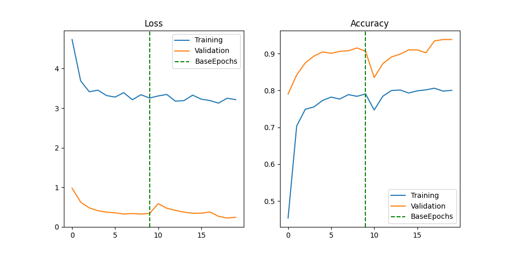
The plot below gives us some interesting insights into how the model training went. We see that the model reaches a relatively strong performance after only a small amount of training epochs, but then seems to starting leveling off. After the fine-tuning kicks in, we then witness a significant drop in accuracy, which suggests that the learning rate was probably too high, triggering too large weight changes within the back-propagation of the network. However, after a couple of epochs, the model is back on track, reaching performance levels which were not attainable earlier.
Looking at the examples from the tensorflow website, we did not spot any drop in accuracy to the extent that we encountered. Unsure whether that problem was only due to a potentially higher learning rate, we tried a range of learning rates, always encountering the same problem. We therefore suspect that the drop of the learning rate is likely going to be a result of having so little training data, compared to the example shown on the tensorflow website, which uses the well-known cats vs. dogs dataset.
Overall we are happy with the model performance, which reaches an accuracy of 93.17% on the unseen test data.
Phone Application
Finally, we thought it would be a nice to deploy the model on a mobile application, as that was also the motivation of choosing the MobileNetV2 network. In order to do so, one has to convert the h5 format the model is currently saved as, into a tflite file. Doing that compresses the model and brings it into the right format for the job. Furthermore, we have to sort and store all the labels into a text file and put them into the Model folder of the application parent folder.
This app folder is pulled from the official tensorflow repository, found here.
sd.seedir("../app/model", style="lines", exclude_folders="__pycache__")
model/
├─.DS_Store
├─oxford_flower_102.tflite
├─labels_flowers.txt
├─mobilenet_quant_v1_224.tflite
├─labels.txt
└─.gitignore
# %% Packages

import json
import tensorflow as tf

# %% Loading models and data

# Model
keras_path = "./models/oxford_flower102_fine_tuning.h5"
keras_model = tf.keras.models.load_model(keras_path)
converter = tf.lite.TFLiteConverter.from_keras_model(keras_model)
tflite_model = converter.convert()
with open("./models/oxford_flower_102.tflite", "wb") as f:
    f.write(tflite_model)

# Labels
labels_path = "./data/cat_to_name.json"
with open(labels_path) as json_file:
    labels_dict = json.load(json_file)
sorted_labels_dict = sorted(labels_dict.items(), key=lambda x: int(x[0]))
label_values = [x[1] for x in sorted_labels_dict]
textfile = open("./models/labels_flowers.txt", "w")
for element in label_values:
    textfile.write(element + "\n")
textfile.close()
After some adjustment in xcode, we can then deploy the app on any iOs device and use the camera for live prediction. The result of which can be seen on the gif below.