How to create Country Heatmaps in R

One of the most powerful visualization tools for regional Panel data there is.

Much of the data that we interact with in our daily lives has a geographical component. Google maps records our favorite places, we calculate how many customers frequent each location for a given brand shop, and we compare eachother by regional difference. Next to bar-charts and line-charts, are there better ways that we can visualize geospatial data? A geographical heatmap can be a powerful tool for displaying temporal changes over geographies.

The question is how to build such a visualization. This tutorial explains how to build a usable GIF from panel data- time series for multiple entities, in this case German states. The visualization problem to which we apply this heatmap GIF is displaying data about the economic development (change in GDP per Capita) of Germany between 1991 and 2019. The data for this example can be found here on our GitHub.

Data Import and Basic Cleaning

To begin with, we import the relevant packages, define the relevant paths and import the needed data. Note that next to the GDP (referred to as BIP in german) per state, we also import the annual inflation rate for Germany using Quandl. The Quandl API provides freely usable financial and economic datasets. In order to use the API we have to create an Account and generate an API-Key, which then has to be specified in the data-generating command.

The reason we need the inflation rate of Germany over the years is that the GDP per Capita is currently in nominal terms, which means that it is not adjusted for inflation and therefore non-comparable between years.

# Packages
library("readxl")
library(Quandl)
library(dplyr)
library(tidyverse)
library(sp)
library(raster)
library(ggplot2)
library(ggthemes)

# Paths
main_path = "/Users/paulmora/Documents/projects/germany_bip_state"
raw_path = paste(main_path, "/00 Raw", sep="")
code_path = paste(main_path, "/01 Code", sep="")
data_path = paste(main_path, "/02 Data", sep="")
output_path = paste(main_path, "/03 Output", sep="")

# Importing data
bip_per_state = read_excel(paste(raw_path, "/bip_states.xlsx", sep=""),
                           skip=10)
german_inflation = Quandl("RATEINF/CPI_DEU", api_key="XXXXXXXX", # Insert API-Key here
                          collapse="annual")

After importing our data, it is now time for some basic data cleaning. This involves reshaping the data, creating the inflation adjusted GDP per Capita figures and creating an unique identifier for each state.

Why exactly reshaping the data is required can be better explained by looking at the raw dataframe, which contains the currently nominal GDP per Capita figures.

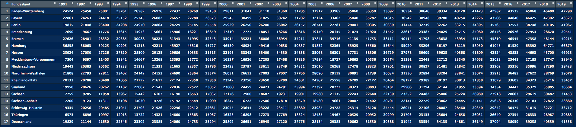
The data representation we face is referred to as a wide-format. A wide-format means that one variable (in that case the year information) is used as columns. Therefore, the entire dataset is much wider than if the variable year would be represented by only one column. This would then lead to a much longer dataset, which is why this format is referred to as the long-format. The change from a wide-format to a long-format is necessary because of our plotting tool ggplot, which could be seen as R’s equivalent to Python’s Seaborn.

Inflation

After knowing why and how we have to reshape the GDP per Capita dataset, it is now time to elaborate on how to process the inflation data. For that we briefly cover what Inflation is and why it is needed.

Inflation describes the measure of the rate by which the average price level increases over time. A positive inflation rate would imply that the average cost of a certain basked of goods increased over time and that we can buy fewer things with the same amount of money. That implies that 100 Euros in 2019 can buy us less than the same amount in 1991. To make these number comparable nevertheless, we have to adjust them for inflation.

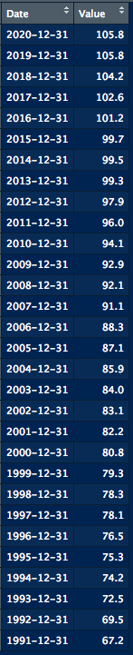
The way we measure inflation is through something which is referred to as the Consumer-Price-Index (CPI). This index represents the price of a certain basket of goods at different points in time. From the data-frame on the left side we can see that this basket cost 67.2 in 1991 and 105.8 in 2020. Given that our GDP per Capita data only ranges until 2019, and that a CPI index is normalized to a certain year, we divide all values of this data-frame by the CPI value in 2019.

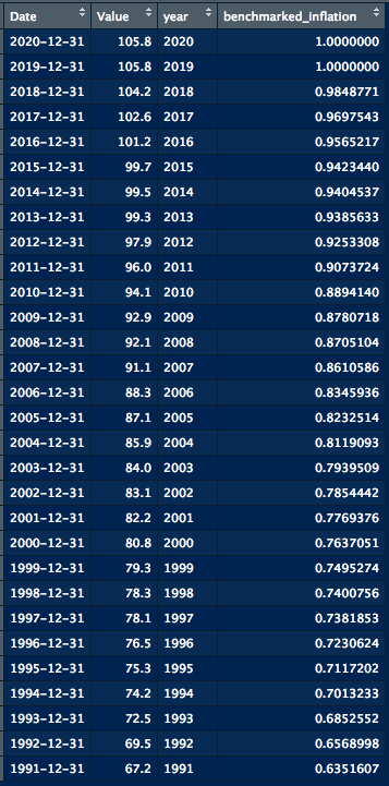
The result of dividing all CPI values by the index-level of 2019 can be seen in the data-frame on the left. Now these values are easier to interpret. An average product in 1991 cost 63.5% of what it cost in 2019.

We can use these values now to adjust the GDP per Capita values over time in order to make them comparable over the years. This is done by simply dividing all GDP values by the respective inflation value of a given year.

Additionally we extract the year information from the Date column in order to match with the year information from the GDP per Capita sheet.

All of the described steps of reshaping and handling inflation are done through the code snippet below.

bip_per_state$id = seq(nrow(bip_per_state))
reshaped_data = gather(bip_per_state, year, gdp, "1991":"2019",
                       factor_key=TRUE)

german_inflation$year = substr(german_inflation$Date, 0, 4)
german_inflation$benchmarked_inflation = (german_inflation$Value
                                          / max(german_inflation$Value))
subset_inflation = german_inflation %>%
  dplyr::select(year, benchmarked_inflation)
gdp_data = merge(reshaped_data,
                 subset_inflation,
                 by=c("year"))
gdp_data$real_gdp_per_capita = gdp_data$gdp / gdp_data$benchmarked_inflation

Importing Geospatial data for Germany

After cleaning our data and bringing it into a ggplot-friendly long-format, it is now time to import geospatial data of Germany. Geospatial or spatial data contains information needed to build a map of a location, in this case Germany.

Importing that information is done through the handy getData function. This function takes, amongst other things, the country name and the level of granularity as an input. In our case we specify “Germany” as the country and because we are interested not only in the country as a whole, but rather in the different states we specify a granularity level which also gives State information. The API gives us a so called Large SpatialPolygonsDataFrame. When opened this object looks like this:

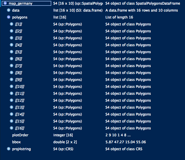
We can see that we find 16 polygons. This makes sense given that we have 16 states in Germany. Each state is therefore represented by one Polygon.

It is important to note that the order of these 16 Polygons does not necessarily align with the alphabetical order of the German states. Therefore, we have to make sure that the information of GDP per Capita is matched up with the right Polygon. Otherwise it could be that we plot the information for e.g. Berlin in Hamburg or vice versa.

Lastly, we have to bring the information into a data frame into the long-format that ggplot prefers. This is done through the broom package, which includes the tidy function. This function, like the entire package, is for tidying up messy datatypes and bring them into a workable format.

The code for the aforementioned steps looks the following:

map_germany = getData(country="Germany", level=1)

from_list = c()
for (i in 1:(nrow(bip_per_state)-1)) {
  id_num = map_germany@polygons[[i]]@ID
  from_list = append(from_list, id_num)
}

to_list = seq(1:(nrow(bip_per_state)-1))
map = setNames(to_list, from_list)

spatial_list = broom::tidy(map_germany)
spatial_list$id = map[spatial_list$id]

The resulting data frame below now shows us all the desired information. The longitude and latitude information (long and lat) is needed for ggplot to know the boundaries of a state and the id column tells us which state we are looking at.

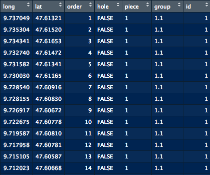
The only remaining steps are to merge the GDP per Capita onto the mapping information and plotting it all.

Plotting

Our final plotting code has to be fine-tuned to fit the purpose of the visualization. In our case, we would like to have one heatmap for every year between 1991 and 2019. To achieve that one could run the plotting code in a loop, iterating over all years, which is also what we will do later on. For better readability though, we start by showing how to plot a single year.

We start by subsetting the GDP per Capita data frame so that it only contains information for a certain year (e.g. 1991). Afterwards, we merge these 16 rows for this single year onto the mapping data frame we showed earlier. The merging variable is the id column we discussed earlier. Afterwards we can already call ggplot and fine-tune our plot.

Germany has two states (Bremen and Berlin) which are fully embedded in other, bigger states. It could therefore happen that the bigger state around them is simply plotted over the smaller state. Therefore it is important to tell ggplot that the bigger states should be plotted before these smaller states, which is also shown in the upcoming code snippet (line 7–11).

gdp_per_year = gdp_data %>% filter(year==1991)
spatial_data_per_year = merge(spatial_list, gdp_per_year, by="id")

gdp_plotting = spatial_data_per_year %>%
  ggplot(aes(x = long, y = lat, group = group)) +
  geom_polygon(aes(fill=real_gdp_per_capita), color="white",
               data=filter(spatial_data_per_year,
                           !Bundesland %in% c("Berlin", "Bremen"))) +
  geom_polygon(aes(fill=real_gdp_per_capita), color="white",
               data=filter(spatial_data_per_year,
                           Bundesland %in%  c("Berlin", "Bremen"))) +
  theme_tufte() +
  coord_fixed() +
  scale_fill_gradient(name="Real Euros per Capita",
                      limits=c(overall_min, overall_max),
                      guide=guide_colourbar(barheight=unit(80, units="mm"),
                                            barwidth=unit(5, units="mm"),
                                            draw.ulim=F,
                                            title.hjust=0.5,
                                            label.hjust=0.5,
                                            title.position="top")) +
  coord_map() +
  ggtitle(paste("GDP Per Capita -", year_num)) +
  theme(axis.title.x=element_blank(),
        axis.text.x=element_blank(),
        axis.ticks.x=element_blank(),
        axis.title.y=element_blank(),
        axis.text.y=element_blank(),
        axis.ticks.y=element_blank(),
        legend.title=element_text(size=25),
        legend.text=element_text(size=20),
        legend.position="right",
        plot.title = element_text(lineheight=.8, face="bold", size=45)) +
  ggsave(paste(output_path, "/maps/", year_num, ".png", sep=""))

The code above will now generate and save the following image:

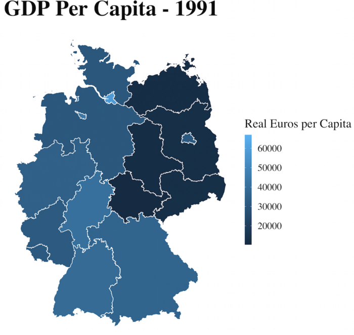
Putting all together into a GIF

If we would now even like to include a time component we could also create multiple heatmaps, one for every year, and play them one after another through a GIF. For that we make use of the beautiful ImageMick package which simply takes all available images in a specified folder and converts them into a GIF.

The following snippet of code shows the procedure to first create heatmaps for all years before turning them into a GIF like it can be seen below.

for (year_num in unique(gdp_data$year)) {

  gdp_per_year = gdp_data %>% filter(year==year_num)
  spatial_data_per_year = merge(spatial_list, gdp_per_year, by="id")

  gdp_plotting = spatial_data_per_year %>%
    ggplot(aes(x = long, y = lat, group = group)) +
    geom_polygon(aes(fill=real_gdp_per_capita), color="white",
                 data=filter(spatial_data_per_year,
                             !Bundesland %in% c("Berlin", "Bremen"))) +
    geom_polygon(aes(fill=real_gdp_per_capita), color="white",
                 data=filter(spatial_data_per_year,
                             Bundesland %in%  c("Berlin", "Bremen"))) +
    theme_tufte() +
    coord_fixed() +
    scale_fill_gradient(name="Real Euros per Capita",
                        limits=c(overall_min, overall_max),
                        guide=guide_colourbar(barheight=unit(80, units="mm"),
                                              barwidth=unit(5, units="mm"),
                                              draw.ulim=F,
                                              title.hjust=0.5,
                                              label.hjust=0.5,
                                              title.position="top")) +
    coord_map() +
    ggtitle(paste("GDP Per Capita -", year_num)) +
    theme(axis.title.x=element_blank(),
          axis.text.x=element_blank(),
          axis.ticks.x=element_blank(),
          axis.title.y=element_blank(),
          axis.text.y=element_blank(),
          axis.ticks.y=element_blank(),
          legend.title=element_text(size=25),
          legend.text=element_text(size=20),
          legend.position="right",
          plot.title = element_text(lineheight=.8, face="bold", size=45)) +
    ggsave(paste(output_path, "/maps/", year_num, ".png", sep=""))
}

setwd(paste(output_path, "/maps/", sep=""))
system("convert -delay 80 *.png maps_over_time.gif")
file.remove(list.files(pattern=".png"))

By tweaking these code snippets, you can create your own geographical heatmaps for other visualization challenges.