
Generative Adversial Networks and Wasserstein Addition
This blog-post elaborates on the workings of Generative Adversial Networks (GANs). Particularly we are looking at the high-level mathematics and intuition of GANs. Furthermore, we are looking into the weaknesses of GANs and proposed enhancements. One development of GANs we are looking deeper into is called the Wasserstein GAN (WGAN), which introduced a new distribution distance function. In the very end of the blog-post we are showing the results of applying such a WGAN model on flag images from all around the world with promising results.
Concept of GANs
Generative Adversial Networks [1], or also known as GANs are all about creating artificial data, which with enough training resembles real data to the extent that neither a machine nor a human can tell the difference between real and fake anymore. This technique allows for sheer endless opportunities in nearly all aspects of our lives. Though, it also creates a debate about ethical usage of such technology, since it will soon be possible to create images which look completely realistic, but are actually the mere product of a machine, so-called deepfakes. This post deals rather with the mathematical idea of GANs than with the ethical questions. That is not because the ethical aspects are in any form less important, but talking about the ethical aspects of such a technology would deserve its own post and not a mere side-note of another one.
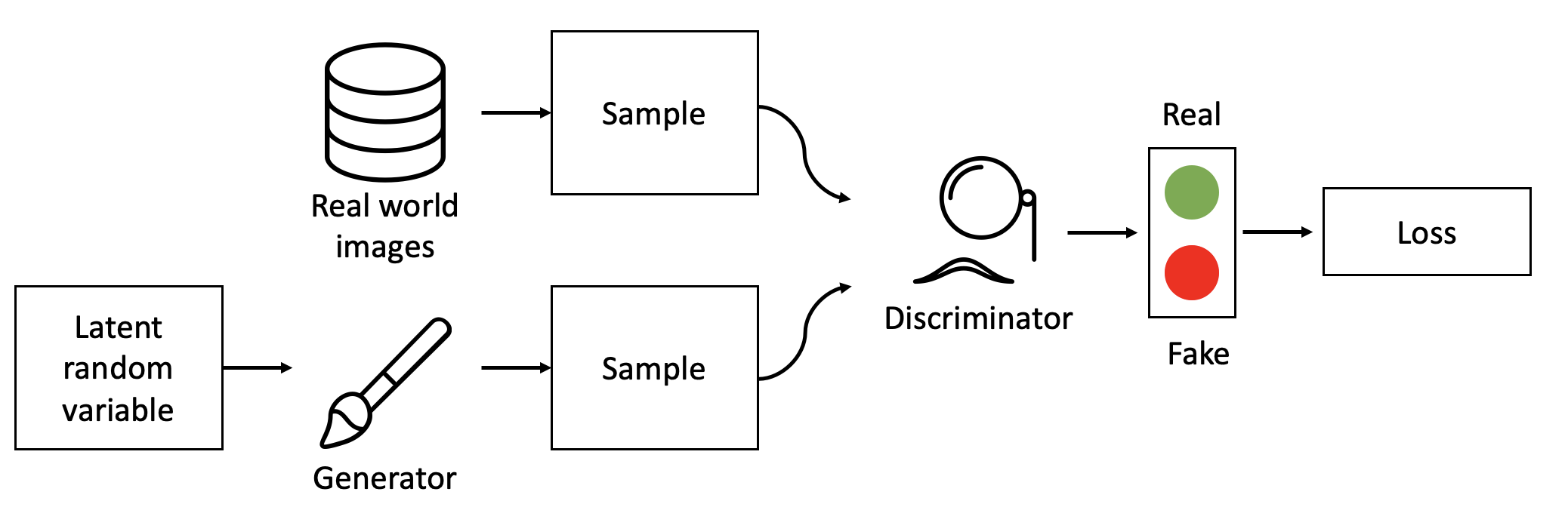
When talking about a GAN, the first thing to understand is that a GAN does not consist out of one model only. In fact there are two models competing with each other. These two models are referred to as Discriminator and Generator. As the name arguably already suggests, the Generator’s job is to create the artificial image, whereas the Discriminator is trying to tell which image belongs to the real images and which one is fake.
The workings of the GAN are oftentimes compared to the never ending battle between art-forgers and the police. In the beginning the art-forgers are very bad at painting. Therefore all of their forgeries are pretty easy to tell apart from Van Gogh’s or Monet’s paintings. Luckily for the art-forgers though, they are always perfectly aware by exactly how much their forgery was away from the quality of a real painting. Based on that information, they update their painting technique and try again. At the same time, the police is also getting better at judging which painting is a fraud and which one is not. In the limits both the police as well as the art-forgers are constantly getting better, and with them, the created forgeries.
This analogy pretty accurately depicts what is happening when training a GAN. It is important to understand that every image, for example the images of national flags, can be described by a probability distribution. This distribution is rather complex and high dimensional. Furthermore, the distribution is also unknown to us. In order to create new flag images, we would have to learn this distribution. There are multiple ways to do so. The arguably most famous ways are Variational Autoencoders (VAE) and Generative Adversial Networks.
Variational Autoencoders, as the name already suggests, encode the real images and break them down into the most important features of the image. Afterwards, these feature are decoded again and it is tried to output the image we initially inputted. Afterwards we are comparing how different the inputted and outputted images are and update our network accordingly. The exact way how the encoding and decoding of a Variational Autoencoder work is left for a future post, since we are focusing more on the second method, namely GANs.
In contrast to VAEs, the general idea of GANs is that if we would like to sample from a complex, high dimensional distribution such as images, we just sample from a simple distribution and apply a transformation to it and through that approximate the complex distribution. This transformation is where neural networks come into play, since they are the perfect tool to approximate complex functions and distributions.
In practice that means that we are using random noise, usually taken from a Gaussian Distribution as the input of the Generator, which then outputs an image. This input vector is referred to as a latent vector. Which number within the input vector is controlling which shape or color from the resulting image is learned by the network alone. Through adjusting the weight parameters, the Generator is then learning which transformation is necessary in order to turn the distribution of the latent vector into the distribution of real images (i.e. how to transform $p_{z}$ into $p_{data}$).
For the Discriminator we are also using a neural network, but with another intent. Instead of starting with random latent vector and outputting an image, we are feeding the flattened image into the Discriminator and output a probability for whether the image is real.
Objective Function of GANs
To get a better feeling how GANs are trained, we take a look at the objective function. The objective function of GANs is slightly different from a standard objective function because we have two models to optimize rather than one. More specifically, whereas the Discriminator would like to minimize the loss of separating real and fake images, the Generator is trying to maximize exactly this loss. The Generator would like the Discriminator to fail.
These objective functions where we have a minimization and maximization problem at the same time, are called minimax functions. In the following function the Generator is denoted as G, and the Discriminator is denoted as D.
\[\begin{align} \min_{G} \max_{D} & \; V(D, G) \\ V(D, G) = & \; \mathbb{E}_{x \sim P_{data}(x)} \left[log(D(x)) \right] + \mathbb{E}_{z \sim P_{z}(z)} \left[1-log(D(G(z)) \right] \end{align}\]$P_{data}(x)$ describes the distribution of the real dataset. $P_{z}(z)$ describes the distribution of $z$, which is usually Gaussian. $G(z)$ describes the output of the Generator when we feed in the vector $z$. Furthermore, $D(x)$ describes the probability that the Discriminator thinks that the input $x$ is real. Equivalently, $D(G(z))$ describes the result of the Discriminator when feeding in the output of the Generator.
In the following we are now rewriting this objective function to gain further insights. We start by replacing the expectation symbols by what they actually stand for, a weighted average. Since we are dealing with a continuous problem, we are using an integral instead a summation sign.
\[\begin{align*} &= \int_{x} p_{data}(x) \; \log(D(x)) \; dx + \int_{z} p_z (z) \; \log(1-D(G(Z))) \; dz \label{eq:rewritten_objective} \tag{1} \end{align*}\]Now we would like to replace every instance of $z$ with an expression of $x$. This is done in order to have fewer variables to work with. This task is easily done after realizing that the data $x$ is nothing other than the output of the Generator which itself took $z$ as an input. Therefore we know:
\[\begin{align} x = G(z) \quad \rightarrow \quad z = G^{-1}(x) \quad \rightarrow \quad dz = (G^{-1})'(x)dx \end{align}\]With these helper equations we can now replace any instance of $z$ in $\eqref{eq:rewritten_objective}$. This step results in the following equation:
\[\begin{align*} &= \int_{x} p_{data}(x) \; \log(D(x)) \; dx + \int_{x} p_z (G^{-1}(x)) \; \log(1-D(x))(G^{-1})'(x)) \; dx \end{align*}\]We note that there is still one $z$ in the equation above, namely $p_z$. In order to also replace this part of the expression we are using a mathematical property of probability density functions. Namely, that if one variable is a monotonic transformation of another variable, then the differential area must be invariant under change of variables.
Digression: Probability density function
If we have a monotonic transformation, for example \(Y = g(X)\), then it follows that \(|f_Y(y) dy = f_X(x) dx|\). That is because that the probability contained in a differential area bust me invariant under change of variables. That is because $f_X(x)dx$ represents nothing other than mass under the density curve. $f_X(x)$ represents the height of the density function and $dx$ the width. A monotonic transformation of the product of height and width of the density function might change the level of height and width, but not the product. Because of the following we can write:
\[\begin{align} f_Y(y) = \left| \frac{dx}{dy} \right| f_X(x) = \left| \frac{d}{dy} (x) \right| f_X(x) = \left| \frac{d}{dy} (g^{-1} (y)) \right| f_X(g^{-1} (y)) = \left| (g^{-1} (y)) \right| f_X(g^{-1} (y)) \end{align}\]Given that we are assuming that the transformation the Generator is applying on the latent vector $z$ is monotonic, we can rewrite $p_z (G^{-1}(x)) (G^{-1})’(x))$ as simply $p_g$. After replacing also the last occurrence of the latent vector $z$, our final equation looks like the following:
\[\begin{align*} &= \int_{x} p_{data}(x) \; \log(D(x)) \; dx + \int_{x} p_g \; \log(1-D(x)) dx \\ &= \int_{x} p_{data}(x) \; \log(D(x)) \; + p_g \; \log(1-D(x)) dx \\ \end{align*}\]After eliminating every occurrence of $z$ within our equation, we now shift our attention to the inner maximization problem. The idea here is that we would like to maximize the objective functions with respect to D. We are maximizing this, since we would like that the Discriminator is able to separate fake and real images.
\[\begin{align} \max_{D} V(D, G) = \int_{x} p_{data}(x) \; \log(D(x)) \; + p_g \; \log(1-D(x)) dx \label{eq:only_x_function} \tag{2} \end{align}\]Maximizing this function means that we have to take the first derivative of that function and set it equal to zero. Note that we are taking the derivative of that function at the position of $x$. Because of that, we are not seeing any integral sign in the equation below.
\[\begin{align} \frac{\partial}{\partial D(x)} p_{data}(x) \; \log(D(x)) \; + p_g \; \log(1-D(x)) &= 0 \\ \rightarrow \frac{p_{data}(x)}{D(x)} - \frac{p_g(x)}{1-D(x)} &= 0 \\ \rightarrow D(x) &= \frac{p_{data}(x)}{p_{data}(x) + p_g(x)} \end{align}\]This result is quite important. It tells us what the optimal level of the Discriminator is for a given Generator. We are now able to use that result and insert it into our objective function in $\eqref{eq:only_x_function}$. We do that in order to find the resulting level of the Generator when using the optimal value of the Discriminator.
\[\begin{align} &= \int_{x} p_{data}(x) \; \log(D(x)) \; + p_g \; \log(1-D(x)) dx\\ &= \int_{x} p_{data}(x) \; \log(D^*(x)) \; + p_g \; \log(1-D^*(x)) dx\\ &= \int_{x} p_{data}(x) \; \log\left( \frac{p_{data}(x)}{p_{data}(x) + p_g(x)} \right) \; + p_g \; \log\left( \frac{p_{g}(x)}{p_{data}(x) + p_g(x)} \right) dx\\ \end{align}\]After getting the equation to that not very intuitive shape, we have to make a mathematically allowed, but strange looking adjustment. Namely, we have to divide and multiply the denominator by positive two. Note that the following equations make use of that fact that $log(\frac{1}{2} \cdot A) = log(A) - log(2)$.
\[\begin{align} &= \int_{x} p_{data}(x) \; \log\left( \frac{p_{data}(x)}{2\frac{p_{data}(x) + p_g(x)}{2}} \right) \; + p_g \; \log\left( \frac{p_{g}(x)}{2\frac{p_{data}(x) + p_g(x)}{2}} \right) dx \\ &= \int_{x} p_{data}(x) \; \log\left( \frac{p_{data}(x)}{\frac{p_{data}(x) + p_g(x)}{2}} \right) \; + p_g \; \log\left( \frac{p_{g}(x)}{\frac{p_{data}(x) + p_g(x)}{2}} \right) dx - 2\log(2) \\ \end{align}\]The equation we arrived at yet is also known as the Kullback-Leibler Divergence (aka KL-Divergence). KL-Divergence is used to quantify the difference of two distributions.
\[\begin{align} &= KL \left[ p_{data}(x) || \frac{p_{data} + p_g}{2} \right] + KL \left[ p_{g}(x) || \frac{p_{data} + p_g}{2} \right] - 2 log(2) \label{eq: kl_divergence} \tag{3} \end{align}\]We are interested in minimizing that quantity with regards to the Generator since if the difference in distribution of $p_g$ and $p_{data}$ is small, we are creating fake data which is very similar to real data.
When trying to minimize the expression above, we have to note that KL-Divergence cannot be negative, as it is a measure of similarity. Therefore we know that expression $\eqref{eq: kl_divergence}$ is minimal when the KL-Divergence parts are equal to zero.
The difference in two distribution is only zero if and only if the distributions of $p_{data}(x)$ (or $p_{g}(x)$) and $\frac{p_{data} + p_g}{2}$ are equal. For that to be the case, the following would have to be fulfilled:
\[\begin{align} KL \left[ p_{data}(x) || \frac{p_{data}(x) + p_{g}(x)}{2} \right] &= 0 \\ \rightarrow p_{data}(x) &= \frac{p_{data}(x) + p_{g}(x)}{2} \\ \rightarrow p_{data}(x) &= p_g(x) \end{align}\]That is a very intuitive result. The Generator reaches its best performance when the distribution of the real data $p_{data}$ is equal to the distribution of the data it creates, namely $p_{g}$.
In fact, equation $\eqref{eq: kl_divergence}$ is describing a special case of KL-Divergence, since both $p_{data}$ and $p_{g}$ are compared to an average of themselves. This special case is called symmetric KL-Divergence. In fact, this phenomena even has its own name, namely the Jenson-Shannon Divergence (aka JS-Divergence). Knowing this, we can rewrite $\eqref{eq: kl_divergence}$ to:
\[\begin{align} &= KL \left[ p_{data}(x) || M \right] + KL \left[ p_{g}(x) || M \right] - 2 \log(2) \\ & \text{where M equals $\frac{1}{2}(p_g(x) + p_{data}(x))$} \\ &= 2 \cdot JSD \left[ p_{data}(x) || p_g(x) \right] - 2 \log(2) \end{align}\]This result tells us, that training the Generator actually means that we are trying to minimize the distance between two distributions. Being able to quantify that distance is important, since we can use it to tell the Generator what went wrong every time it created new images.
The many problems of GANs
Generative Adversarial Networks are an incredible strong tool for many tasks. Though, they are also famous to be very instable. That problem arises because of multiple reasons, some of which are discussed in this section.
Optimizing two functions at a time
One of the biggest problem is the aim to optimize two models in an iterative process. As we already know, GANs are build iteratively. That means that Discriminator and Generator update their weights after one another, not taking the other model into consideration. Salimans et al 2016 describe training a GAN rather fittingly with finding a Nash Equilibrium to a two-player non-cooperative game. A Nash Equilibrium describes a situation in which in neither player has an incentive to unilaterally deviate from their strategy. That means that the Discriminator and Generator have both minimum loss with respect to their weight parameters. The problem is that on the way to a minimum, every change of the Discriminator’s weight parameters can increase the loss of the Generator and vice versa.
Salimans et al. 2016 then also present a very intuitive example to illustrate that argument. Let us assume that the Generator has influence on $g$ in order to minimize the expression $f_g(g) = gd$, whereas the *Discriminator can control $d$ in order to minimize the expression $f_d(d) = -g*d$.
When minimizing a function within gradient descent we are taking the derivative of that function and multiply the result by the learning rate in order to go a step towards the minimum of that function. The derivative of these functions respectively is:
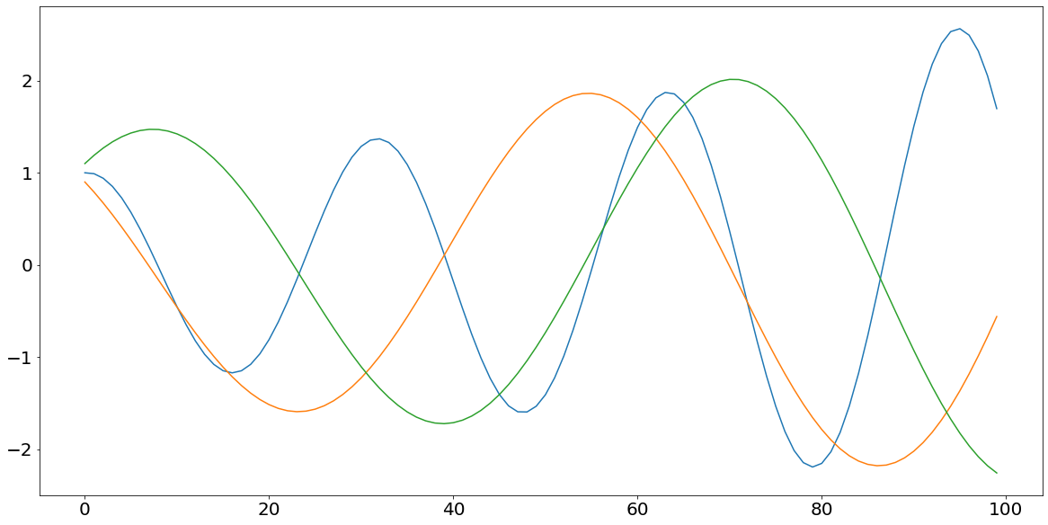
\[\begin{align} \frac{\partial f_g}{\partial g} &= -d \\ \frac{\partial f_d}{\partial d} &= g \\ \end{align}\]After knowing what the partial derivative of the two functions are, we can now go ahead, multiply the result with the learning rate $\eta$ (assumed to be 0.1) and add it to the prior level of $g$ and $d$ respectively. The following snippet of code implements our problem and also shows the result of that function.
As we can see the resulting function $g*d$ is oscillating with an ever growing amplitude, which gets worse over time and contributes substantially to the instability of the model.
import matplotlib.pyplot as plt
import _config

d = g = 1
f_d = d * g
learning_rate = 0.1
f_d_list, d_list, g_list = [], [], []

for _ in range(100):
    d_new = d + learning_rate * g
    g_new = g - learning_rate * d
    f_d = d * g

    d = d_new
    g = g_new

    d_list.append(d)
    g_list.append(g)
    f_d_list.append(f_d)

fig, axs = plt.subplots(figsize=(20, 10))
axs.plot(f_d_list, label="g*d")
axs.plot(g_list, label="g")
axs.plot(d_list, label="d")

plt.show()
Vanishing Gradients
Another common problem of GANs are vanishing gradients. This problem describes the situation in which the Discriminator is doing too good of a job. In the most extreme case we would have a perfect Discriminator which would detect every real sample $D(x) = 1, \forall \; x \in p_{data}$ as real, and every fake image as fake $D(x) = 0 \forall x \; \in p_g$.
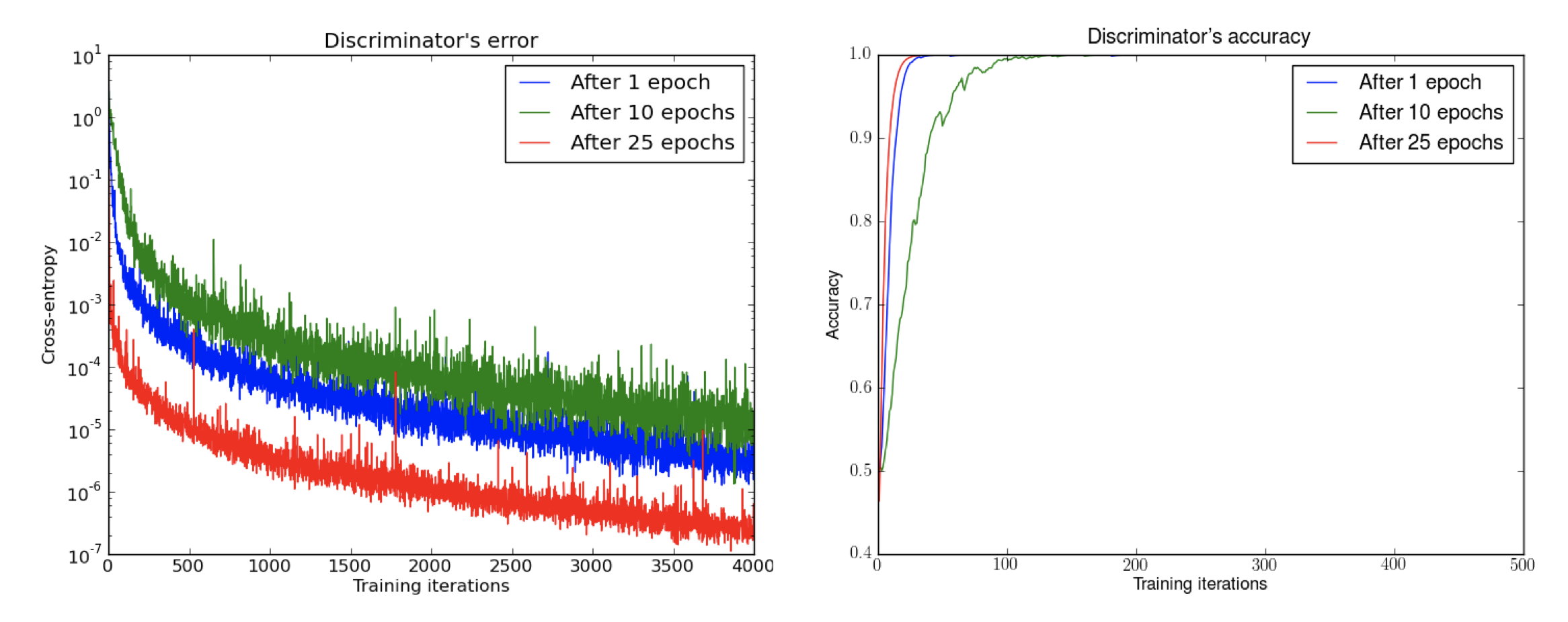
First, we trained a DCGAN for 1, 10 and 25 epochs. Then, with the generator fixed we train a discriminator from scratch. We see the error quickly going to 0, even with very few iterations on the discriminator. This even happens after 25 epochs of the DCGAN, when the samples are remarkably good and the supports are likely to intersect, pointing to the non-continuity of the distributions. Note the logarithmic scale. For illustration purposes we also show the accuracy of the discriminator, which goes to 1 in sometimes less than 50 iterations. This is 1 even for numerical precision, and the numbers are running averages, pointing towards even faster convergence. Source: Arjovsky and Bottou, 2017
This problem leads us to a situation in which the speed of learning is seriously dampened, or even completely stopped. That is because the Discriminator is sending not enough information for the Generator to make any progress, meaning that the Generator does not know how to improve.
Mode collapse
Another problem of GANs are so-called Mode collapses. A mode describes one possible output of the real samples. For example, the MNIST dataset, which contains images of 10 hand-written digits, contains 10 modes.
A mode collapse then describes a situation in which the Generator found a way to produce one or a very limited amount of samples to produce, which the Discriminator is unable to reject. The result of that situation is that the Generator is constantly producing the same subset of data and does not even try to significantly change it anymore, since the Discriminator got stuck in a local minima and does not send meaningful feedback anymore.
The example below shows how the Generator at some point started to solely produce images from the same mode.
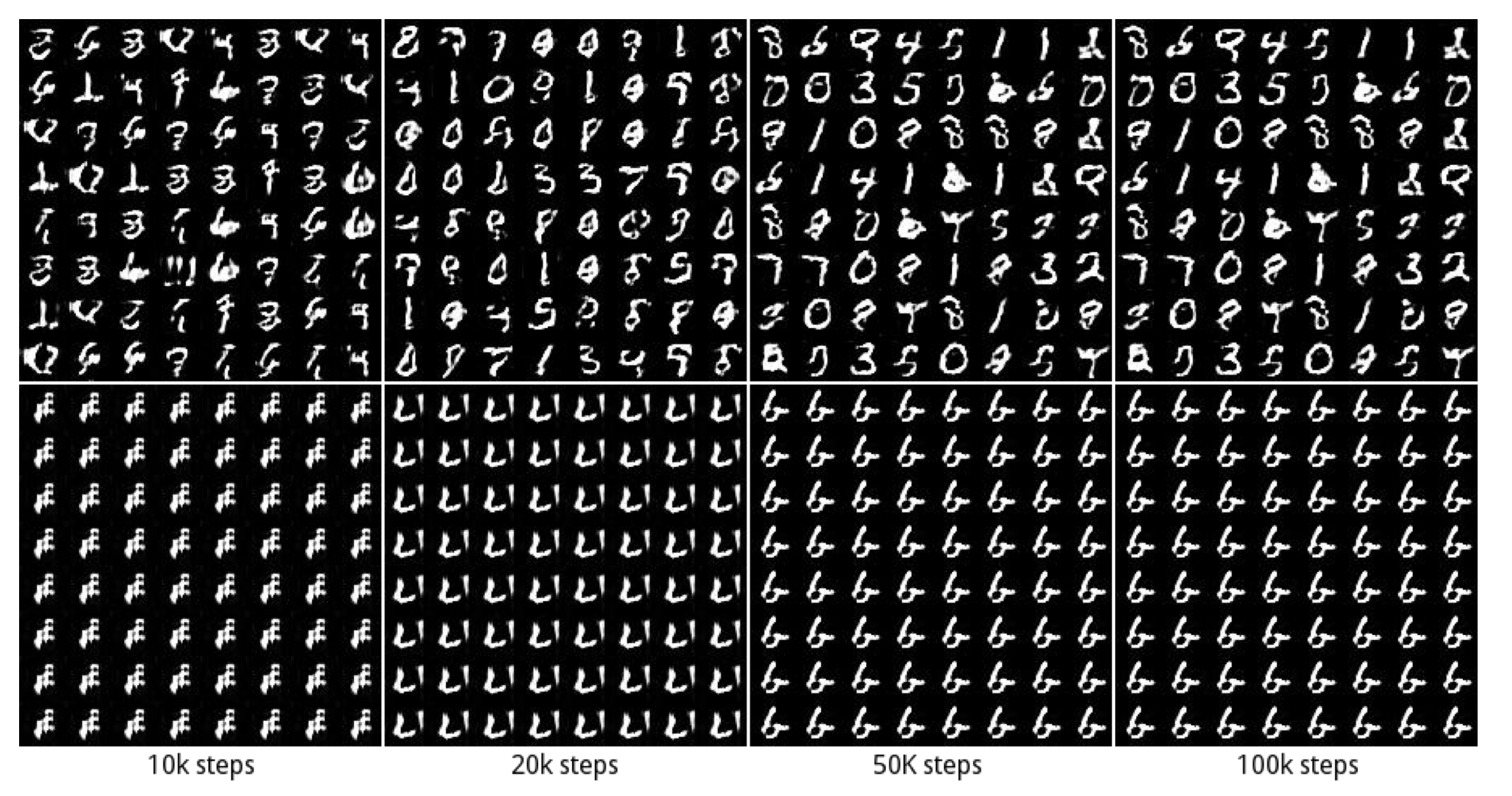
Source: Metz, Luke, et al.
Wassterstein GAN
One solution to the last two problems would be to use a different solution of to measure the distance between $p_g$ and $p_{data}$, called Wasserstein Distance and the resulting Wasserstein GAN [3].
Motivation of Wasserstein Distance
Before starting to talk about how this new distance functions works, we start by motivating why we would even need a different distance measure next to JS-Distance and KL-Divergence. The reason for that is that both the JS and KL distance are quite bad in scenarios where the two distributions are relatively far apart.
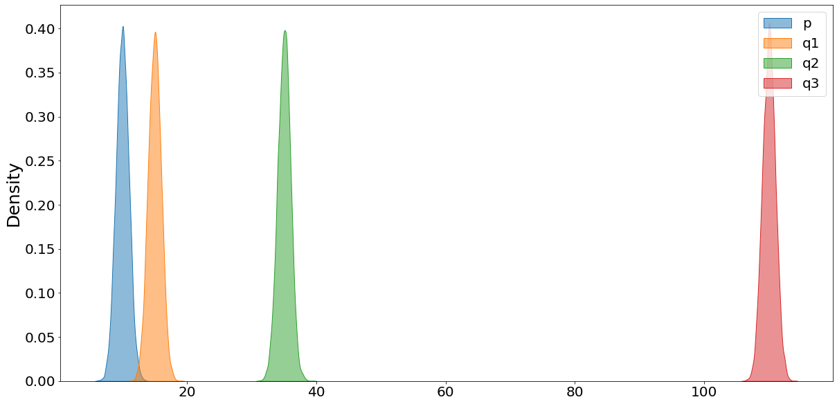
In the following we illustrate what is meant by that. We do that by comparing a distribution called p (shown in blue) with three other distributions whose means are 5, 25, and 100 units away. (Note that we shift all distributions ten units to the right, in order to mitigate negative and zero values. That is necessary since the KL-Divergence cannot handle negative values.)
import numpy as np
import seaborn as sns

BASE_LEVEL = 10
SIZE = 10_000
RANDOM_STATE = 42

data_dict = {
    "p": np.random.normal(loc=BASE_LEVEL, size=SIZE),
    "q1": np.random.normal(loc=(BASE_LEVEL+5), size=SIZE),
    "q2": np.random.normal(loc=(BASE_LEVEL+25), size=SIZE),
    "q3": np.random.normal(loc=(BASE_LEVEL+100), size=SIZE)
}

fig, axs = plt.subplots(figsize=(20, 10))
for key, value in data_dict.items():
    sns.kdeplot(value, label=key, ax=axs, fill=True, alpha=0.5)
axs.legend()
plt.show()
Now we are calculating the KL- and JS-Divergence between the base-distribution (blue) and the other three. Note that we are using rel_entr instead of kl_div, given that the latter is slightly different implemented to the definition of KL-Divergence we used earlier.
from scipy.spatial.distance import jensenshannon
from scipy.special import rel_entr
from scipy.stats import norm

ITERATIONS = 5_000

kld_list = []
jsd_list = []
x1 = norm.rvs(loc=BASE_LEVEL, size=SIZE, random_state=RANDOM_STATE)
for i in range(0, ITERATIONS, 5):
    x2 = norm.rvs(loc=(BASE_LEVEL+i), size=SIZE, random_state=RANDOM_STATE)

    jsd = jensenshannon(x1, x2)
    jsd_list.append(jsd)

    kld = np.abs(np.sum(rel_entr(x1, x2)))
    kld_list.append(kld)

stand_jsd_list = np.array(jsd_list) / np.max(jsd_list)
stand_kld_list = np.array(kld_list) / np.max(kld_list)

fig, axs = plt.subplots(figsize=(20, 5))
axs.plot(stand_kld_list, label="KL-Distance", color="black")
axs.plot(stand_jsd_list, label="JS-Distance", color="purple")

for name, dist, color in zip(["q1", "q2", "q3"], [5, 25, 100], ["orange", "green", "red"]):
    axs.vlines(x=dist, ymin=0, ymax=1, linestyles="dashed", label=name, color=color)
axs.legend()
plt.show()
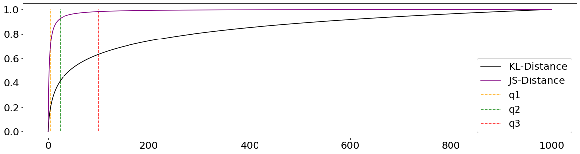
As we can see from the chart above, both, the KL- and the JS-Divergence level out fairly soon. This represents a problem since the Generator is not getting enough information in order to meaningful improve. It is not sufficiently communicated how bad/good of a job the Generator is doing. That leads then to a situation where the gradient is close to zero and the Generator is not able to learn anything.
from scipy.stats import wasserstein_distance
wasserstein_list = []
for i in range(0, ITERATIONS, 5):
x2 = norm.rvs(loc=(BASE_LEVEL+i), size=SIZE, random_state=RANDOM_STATE)
wd = wasserstein_distance(x1, x2)
wasserstein_list.append(wd)
stand_wasserstein_list = np.array(wasserstein_list) / np.max(wasserstein_list)
fig, axs = plt.subplots(figsize=(20, 5))
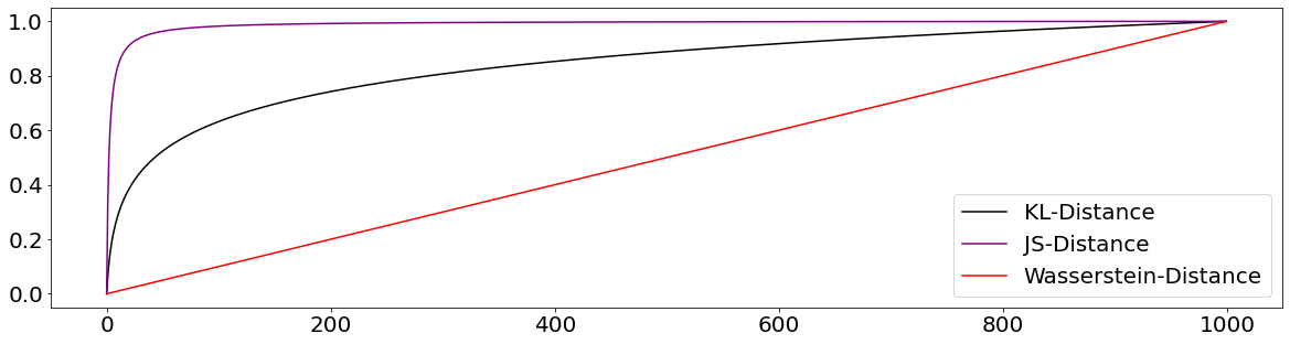
axs.plot(stand_kld_list, label="KL-Distance", color="black")
axs.plot(stand_jsd_list, label="JS-Distance", color="purple")
axs.plot(stand_wasserstein_list, label="Wasserstein-Distance", color="red")
axs.legend()
plt.show()
What exactly is the Wasserstein Distance
From the chart above we can see why we would rather use the Wasserstein Distance to assess the similarity between two distributions. In contrast to KL- and JS-Divergence, the Wasserstein Distance provides us with a nicely scalable way to assess the similarity between two distributions.
The Wasserstein Distance is also called the Earth Mover’s Distance, given that it can be interpreted as the minimum amount of effort of transforming one distribution into the shape of another distribution. Effort is defined here as the amount of probability mass times the distance we are moving the mass.
The general workings of this distance measure become clearer when considering a discrete example. We consider two discrete distributions $A$ and $B$, which both have 14 probability mass units (14 is just a random number here). These probability mass units are divided on the four different piles in the following way:
\[\begin{align} A_1 &= 5, A_2 = 2, A_3 = 2, A_4 = 5 \\ B_1 &= 3, B_2 = 3, B_3 = 5, B_4 = 3 \end{align}\]Of course, there are multiple ways how we could transform these two distributions in order for them to match up. There are even more possible transformations with the smallest effort. In the following we are showing one potential way of how to do it, but be aware that there could be more than just that one.
When trying to transform distribution $A$ into distribution $B$ with the smallest amount of effort, the following steps are possible:
- Move 2 units from $A_1$ to $A_2 \rightarrow A_1$ and $B_1$ match up
- Move 1 units from $A_2$ to $A_3 \rightarrow A_2$ and $B_2$ match up
- Move 2 units from $A_4$ to $A_3 \rightarrow A_3$ and $B_3$ & $A_4$ and $B_4$ match up
The overall costs of transforming distribution A into distribution B is then equal to five. This was calculated by simply adding up the number of probability mass units moved (since they were all moved a distance of one respectively). More generalizable, one could use the formula \(W = \sum |\sigma_i|\), in which \(\sigma_{i+1} = \sigma_{i} + A_i - B_i\). Using this formula, the calculation would look the following way:
\[\begin{align} \sigma_0 &= 0 \\ \sigma_1 &= 0 + 5 - 3 = 2 \\ \sigma_2 &= 2 + 2 - 3 = 1 \\ \sigma_3 &= 1 + 2 - 5 = -2 \\ \sigma_4 &= -2 + 5 - 3 = 0 \\ \rightarrow W &= \sum | \sigma_i | = 5 \end{align}\]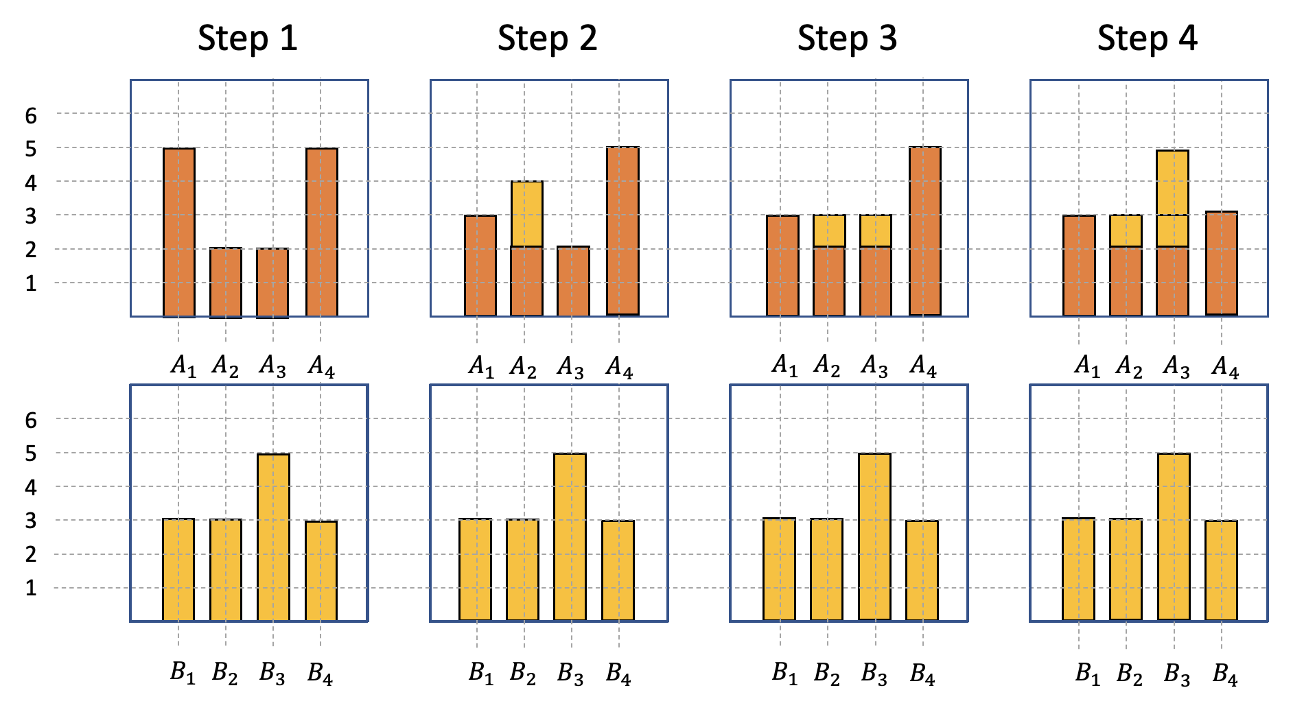
In the continuous case, this formula changes to:
\[W(p_r, p_g) = \underset{\gamma \in \prod(p_r, p_g)}{inf} E_{(x, y) \sim \gamma} \left[ || x- y ||\right]\]This formula describes the very same concept we had for the discrete case, but now for a continuous version. The infimum operator describes that we are interested in the greatest lower bound, hence the smallest effort of transforming distribution x to distribution y.
Given that there is not one way of how to transform distribution x and y in order to match these two distributions, we are considering all possible combinations. That fact is denoted by $\prod (p_r, p_g)$. On the other hand, ||x-y|| describes the distance that we have to push probability mass of x, in order to align with the distribution of y. Lastly we have $\gamma (x, y)$ which describes the percentage of probability mass of x that would be needed to move around in order to align with distribution of y. When multiplying the percentage of distribution mass that is needed to be moved with the distance the probability mass would have to move we would arrive at the formula above:
\[\sum_{x, y} \gamma (x, y) ||x-y|| = E_{(x, y) \sim \gamma} ||x-y||\]It is to be said though calculating all possible combinations is not tractable to calculate all possible combinations of how to match up the two distributions. Meaning that $\prod (p_r, p_g)$ is too large. The authors of the WGAN paper [4] therefore come up with a transformation based on the Kantorovich-Rubinstein duality. This transformation changes our formula to:
\[W(p_r, p_g) = \frac{1}{K} \underset{||f||_L \leq K}{sup} E~p_r \left[f(x) \right] - E~p_g \left[f(x) \right]\]Herein we are using the so-called supremum, which is the opposite of the infimum, meaning that we are interested in the maximum value. Furthermore, the newly introduced function \(f\) is demanded to satisfy $||f||_L \leq K$, which means it should be K-Lipschitz continuous.
Digression: Lipschitz continuity
A Lipschitz continuous functions is nothing other than a continuous function with a limited slope parameter. That becomes clearer when taking a look at the mathematical definition. A function is said to be Lipschitz continuous if $|f(x) - f(y)| \leq L \cdot |x-y| \quad \forall x, y \in \mathbf{R}$
If we now apply a simple transformation for that formula and ensure that $x \neq y$, then we find that
\[\begin{align} |f(x) - f(y)| \leq L \cdot | x-y | \\ \left| \frac{f(x) - f(y)}{x-y} \right| \leq L \end{align}\]From the left side of the formula above we see that this is nothing other than the slope parameter of the function, which in the limits of x converging towards y represents the derivative of the function.
How exactly that Lipschitz continuity is applied to the Wasserstein distance formula is heavy mathematics and not scope of this blog-post. The appendix of the original paper sheds some light on the derivation for those who are interested. If we now consider that the function $f$ is obeying the K-Lipschitz restriction, then we find that the Wasserstein distance is defined as:
\[W(p_r, p_g) = \underset{w \in W}{max} E_{x ~ p_r} [f_w(x)] - E_{z~p_r(z)}[f_w(g_{\theta}(z))]\]In which $f_w$ is K-Lipschitz continuous. Ensuring this Lipschitz continuity during training is difficult, and even the original paper is struggling to do so, suggesting to clip the gradient updated weights between [-0.01, 0.01]. The authors even state in the original paper -Weight clipping is a clearly terrible way to enforce a Lipschitz constraint -. This clipping of parameters also does not completely resolve the problem of vanishing gradients and slow convergence, since the hard-coded clipping of the weights cannot solve all problems.
Since then there were multiple suggestions of how to work-around this problem, the most famous one working with a gradient penalty [4].
Results from using a WGAN
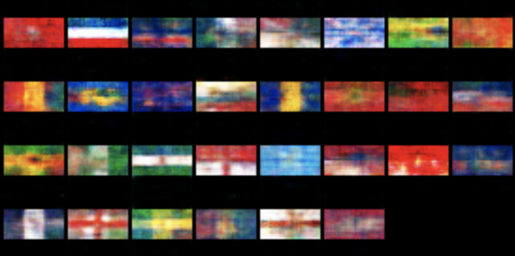
After the theoretical explanation of GAN and WGAN we implemented a working example into Python, using PyTorch. Herein we used flag images from countries all around the world with the aim to create new ones.
We obtained the flag images from here. Given the small amount of images (~250) we applied heavy data augmentation on the images. For this example we implemented the described WGAN, given its better performance over the standard GAN.
From the image below we can see the resulting flags. Even though many of them are not on the level to be used as the new national flag of any emerging country, but the result is still satisfying, considering that these flags were literally created out of random-noise.
Reference List
[1] Goodfellow, Ian J., et al. “Generative adversarial networks.” arXiv preprint arXiv:1406.2661 (2014).
[2] Salimans, Tim, et al. “Improving GANs using optimal transport.” arXiv preprint arXiv:1803.05573 (2018).
[3] Arjovsky, Martin, Soumith Chintala, and Léon Bottou. “Wasserstein generative adversarial networks.” International conference on machine learning. PMLR, 2017.
[4] Gulrajani, Ishaan, et al. “Improved training of wasserstein gans.” arXiv preprint arXiv:1704.00028 (2017).