
Clustering Real Estate Data
Using unsupervised learning techniques to create features for supervised price prediction.
01 What is clustering and what can it be useful for
Clustering has many applications. Most people know it as an unsupervised learning technique. Here, we use clustering to find similarities in observations of real estate listings and allocate similar observations into buckets, but clustering can also be used for other use cases like customer segmentation.
Whenever a new property comes on the market, the question of how it should be priced naturally arises. One good approximation for that is to see how similar properties are priced. The goal here is to define what exactly makes one property similar to another. Clustering can be helpful here to identify which larger category of properties a given property belongs, and which features influence belonging in this category. One can then use the average from this category to get an indication of the price.
Another use case for clustering is to use the cluster information as an additional feature within a supervised prediction model. The reason why that could be a helpful is that a cluster variable provides condensed information to the model. A tree model, for example, has an easier time splitting observations based on one variable instead of splitting based on many variables individually.
To explain that in more depth, let us assume a Random Forest model, which is a special form of bagging. It is special in the sense that it does not consider all features for every tree, but chooses random features for every tree. If a tree chooses the features number of bathrooms and bedrooms but not the number of square meters, it has an incomplete picture. Even though the Random Forest model tries to average out this incompleteness through a majority vote of trees, the tree would have an easier time to have variable which condenses much of the basic information of the property already. That would lead to fewer misclassifications of properties which show an unexpected value for one of their features.
A more elaborate post on the usefulness of using a cluster variable within a supervised predction model is shown here.
02 Clustering Method - K Means
The clustering method used in this example is K Means. The reasons for choosing that clustering method compared to more complicated methods are:
- Simplicity - K Means, compared to many other clustering methods, is relatively easy to understand and to implement. Given that clustering is used as a simple additional feature, the use case does not require an overly complex model.
- Adaptive approach - The algorithm is known to easily adapt to new observations. This means that newly added data can easily classified with this algorithm
- Guaranteed convergence - by trying to minimize the total SSE as an objective function over a number of iterations.
Before jumping into any results it is important to elaborate a bit more on how the K Means algorithm works. The first step, and at the same time one of the most difficult steps within this approach, is to set how many clusters we want our data to be split into. This is challenging - how are we supposed to know how many clusters the data needs? We will elaborate a bit later on how to make an educated guess on that number. For now, we will simply call that mysterious number of clusters k.
We start by taking k randomly selected observations from our dataset. In our case, we choose k randomly chosen properties. These are our initial centroids. A centroid a fancy name for the mean of a cluster. Given that this is our first observation within each cluster, it therefore also represents the mean. Afterwards, we assign all other properties left (N-k) to exactly one of the k groups. This is done by calculating the difference between the features of a property to all possible centroids. Having more than one feature requires us to use the euclidean distance for that. The euclidean distance is the square root of the sum of all squared features of a property.
After we have assigned all properties to one cluster, we re-calculate the means (centroids) of each of the k groups. This is done by calculating the simple average of all observations for each cluster. This calculation marks the end of the first iteration.
The next iteration starts again by allocating all properties to one of the k centroids again, using the euclidean distance of each property. It could now be that some observations which were assigned to a certain group change over to a different of the k groups. If that happens, that means that the model has not yet converged and needs more iterations.
After many iterations, no observation will change its group assignment anymore. When that happens, the algorithm is done and said to have converged. This also means that the summed variation of all k groups has reached a minimum. K Means is heavily dependent on which initial values were randomly chosen at the start. In order to test the robustness of the result, it is advised to apply algorithms such as k-means seeding. These methods test different initial values and assess the change in results.
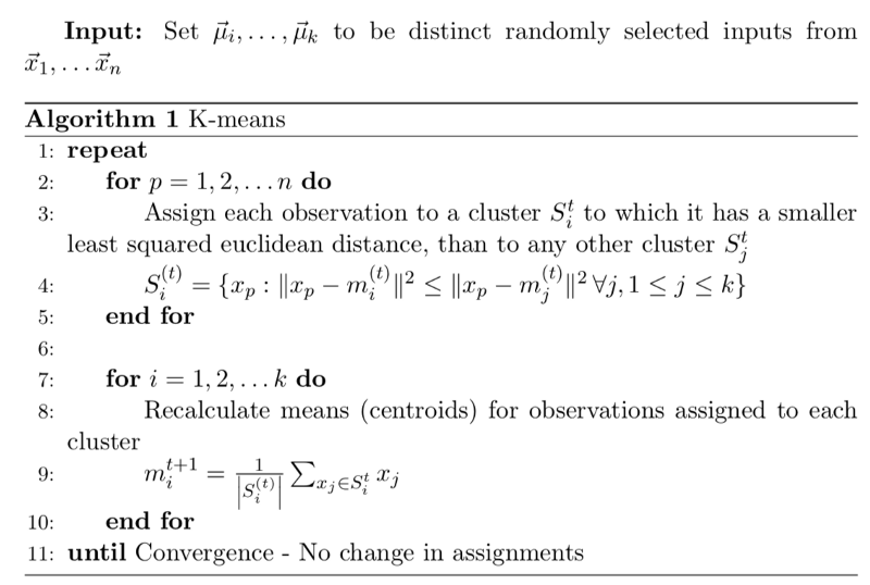
The entirety of the explanation above can also be summarized in the pseudo code below:
02.1 Choosing K
As stressed before, one disadvantage of clustering is the necessity of choosing the number of clusters at the start. This task seems truly difficult since it somewhat requires us to have an initial idea about the data. For cases where we have up to three variables, this problem can be solved by simply plotting the observations and see visually which number of clusters could be sensible.
There are multiple problems with that approach, however. The main problem is probably that “eyeballing” the number of clusters to use based on a plot is not very scientific and very subjective. A more sophisticated approach is the silhouette score, which is explained in the next section.
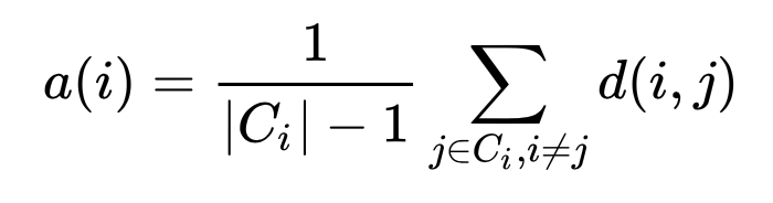
On a high level, what the silhouette score does is to assess whether an observation fits nicely to a certain cluster and badly to a neighboring cluster. This is done through the comparison of two distance measurements. The first is the measurement of how far an observation within a certain cluster is away from the other observations within the cluster. This is done by calculating the average euclidean distance of one observation i to all other observations within the same cluster.
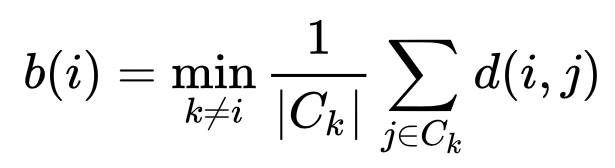
The second measurement is to see how well an observation in a certain cluster fits to all other observations within a so called “neighboring cluster”. A neighboring cluster is the cluster which, on average, is closest to a another cluster. The assessment is done by calculating the average distance of a certain observation to all other observations of a neighboring cluster.
The last step is then to compare these measurements. The silhouette score is defined for a certain observation as the difference between the average distance to a neighboring cluster and the average distance within its cluster. This number is standardized by dividing the difference by the maximum of a(i) and b(i).
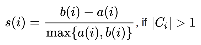
Through this standardization the silhouette score will be between -1 and 1. In order to assess how well the clustering fits not only one observation, but the entirety, the silhouette score is calculated for all observations and then averaged. In our example the average silhouette score for all observations has the following shape:
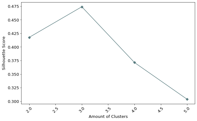
From the graph above, we can see that the best silhouette score is achieved by having three clusters. This result is interpreted as follows: Having three clusters, on average, the mean euclidean distance between an observation and a neighboring cluster is greater than the mean euclidean distance between an observation and other observations within the same cluster.
02.2 Code Implementation
When implementing K Means, it is important to start by figuring out which value k should take using the silhouette score.
# Number of maximum clusters tried
max_cluster = 5
# Initialise dictionary
sil_graph = {}
# Looping starting with 2 clusters and then
for cluster in range(2, max_cluster + 1):
    # Calculate the kmeans with clusters
    kmeans = KMeans(n_clusters=cluster, random_state=0).fit(data)
    # Calculate the kmeans labels
    sil_graph[cluster] = silhouette_score(data_v3, kmeans.labels_)
As seen above, when implementing the silhouette score, we have to state the number of clusters from the start. For our example we tried all cluster levels up to 5. It is important to allow for a relatively high amount of potential clusters. Otherwise, it could happen that the calculation will be only able to find a local minimum.
The second step is then to implement the K Means algorithm with the optimal value of clusters, namely three. This is relatively easy and shown below.
# Choosing decided cluster level
cluster_level = 3
# Initialising cluster level
kmeans = KMeans(n_clusters=cluster_level, random_state=0).fit(data)
# Assign cluster labels
cluster_label = kmeans.labels_
It should be said that before feeding the observations in any of the clustering algorithms, it is advised to first standardize the data. This ensures comparable scaling of the variables.
03 Clustering Results
After deciding for three clusters, it would be interesting to see how the data was split. As discussed before, plotting the variables and highlighting the cluster gets difficult whenever more than three variables are at play.
One workaround is the usage of Principal Component Analysis (PCA). What PCA does is to compress the information of many variables in a selected amount of fewer variables. The graphic below shows exactly that - here, we have projected all the feature variables onto a 2-dimensional plane for plotting.
First, the variables #of bathrooms, # of bedrooms, # of squaremeters, longitude and latitude are used to build exactly two principal components. Afterwards these two newly created variables are plotted. The color of each point shows its assigned cluster group.
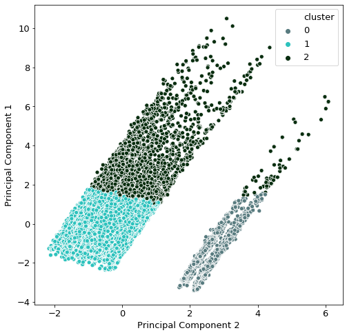
At first glance, the clusters don’t look very intuitive. It seems that we have two islands of observations, one larger than the other.
Given that we are in possession of the location data of the properties, it is also interesting to see how the clustering is spread through the country. One very interesting observation here is that the grey-blue dots are mostly solely in Gran Canaria, whereas all other observations are in Peninsular Spain. This finding explains the two “islands” seen in the original PCA graph.
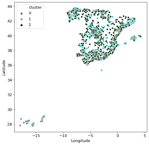
The other mystery that remains now is what causes the two cluster groups within Peninsular Spain. This can be explained with the other variables. The 3-D plot below shows the other 3 features and shows that the cluster group one shows more extreme values for all variables compared to cluster group two.
04 Conclusion
In this post, we explained what clustering can be used for, how the relatively simple method of k-means works, and how to determine k. Furthermore, we showed example code of how to implement the clustering, and the results of clustering our real estate features. We further showed methods of how to visualize the results of clustering.
In the upcoming posts we will use the cluster group as a feature in our prediction model. So stay tuned to read about the performance of this variable!