Multi-label Genre Predictor with Interactive Dashboard
An intuitive explanation of how to deal with a multi-label classification problem using ImdB movie-data.
This blogpost walks through the entire process of building a genre prediction model, using movie descriptions as the sole feature.
This post is structured as follows: We start by giving some background information about the origin of the data and show an example of what information can be extracted from ImdB. Afterwards, pre-processing of the movie descriptions is explained in detail, including an elaborated section on the workings of tfidf-vectorization.
Next, we explain how we dealt with movies which are labelled with more than one genre and motivate our modeling choice. Lastly, we present our results in a custom-build web application designed for this project. The app can be accessed here.
Data Origin
As shown in the last blog post, the movie data was scraped from the ImdB website. We scraped approximately 200k movies with their genre as well as with their descriptions.
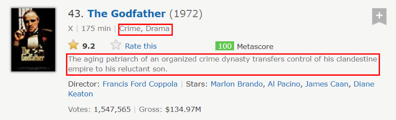
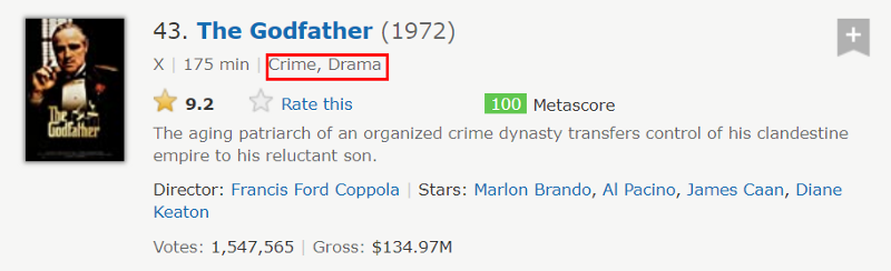
Below we see an example of what information is extracted for each movie. The scraped information is indicated with a red square and consist out of the movie genres as well as the movie descriptions.
Data Processing
Before we can feed any model the movie descriptions, some pre-processing is necessary. Specifically, we must transform the current movie description into some form of numeric representation, in order for the model to use that information. In total we apply four pre-processing steps, outlined below:
- Tokenizing
- Removing stopwords
- Stemming
- Tf-idf vectorization
All four bullet points contain some sort of buzzwords. In the following we will go over each of them and explain what they mean.
Tokenizing describes the process of breaking down the text into its smallest components, called tokens. Tokens are generally words, but can also be numbers of punctuation. Combined, tokens represents the building blocks which give text its meaning. Stop-words are a list of words which are removed from the text, since they carry no information. Stop-words refer to the most common words in a language, or used in a particular setting. Specifically because they are so commonly used everywhere, they do not tend to care any significant information and can therefore be removed in order to allow the model to focus on the more important tokens. Stemming is one of two methods (the other is called lemmatization) to reduce a word to its so called root. The roots of words contain the majority of the meaning. That procedure is best explained by looking at an example. Consider the following two made up sentences:
…he was in quite some trouble… …she was troubled by what she witnessed…
Reading the two sentences, a human being can tell that even though the two words trouble and troubled are not the same word, they carry a similar meaning. A machine, on the other hand, does not know that these two words should be treated as similar or even the same, since they are spelled differently and thus represent two different tokens.
One way to help the machine is to break down each word into its root. Using the NLTK Python package for stemming, this break-down would mean the following for our example:
trouble → troubl troubled → troubl
The example above shows two things. First, both words are identical after the stemming. That is great news for the model, since now it will know that the meaning is the same. The second observation is that the resulting word is not really a word anymore. Exactly here lies the difference between stemming and lemmatization. Stemming does not require that the resulting string carry any meaning for a human reader, whereas lemmatizing always returns a word that actually exists in the language.
Pre-Processing Example
At this point it would make sense to take a look what all pre-processing steps up until now have done to our text. Below we see what our pre-processing has done to the movie description of our example description of The Godfather (1972).
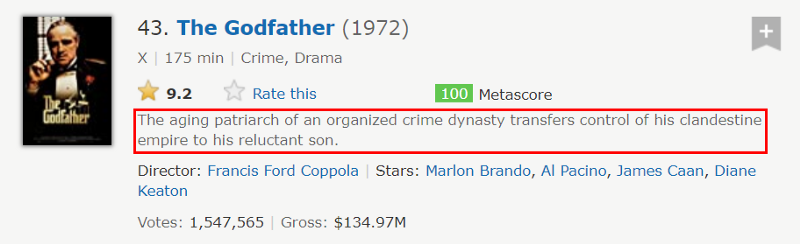
Raw: The aging patriarch of an organized crime dynasty transfers control of his clandestine empire to his reluctant son. Processed: age patriarch organ crime dynasti transfer control hi clandestin empir hi reluct son
The result is hardly readable anymore. Especially the stemming took its toll on readability, reducing every word to its word-stem.
Term frequency-inverse document frequency
The last step on our pre-processing list if tf-idf vectorization. Since this method represents an important step and is not as straight forward to explain as the other pre-processing steps, we will explain that approach in a bit more detail.
The main motivation for the tfidf- vectorization is the translation of the string format of the movie description into a numeric representation of this text. This is necessary given that the prediction-model needs a numeric input.
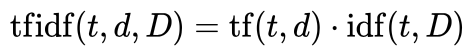
One way to transform a combination of strings into a numeric vector is a methodology called term frequency-inverse document frequency, or tf-idf for short. It represents a ratio of how often a string appears in a given document, compared to how often that word appears in all documents.
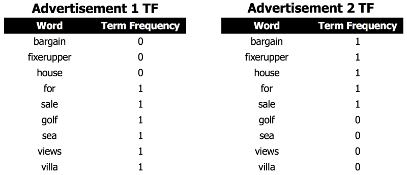
To understand how tfidf vectorization works, we’ll look at a simplified example from the real estate world. In our example, we have 2 short real estate advertisement descriptions where stop-words have been removed.

Note that Advertisement 1 contains 6 words, whereas Advertisement 2 only contains 5 words. Both advertisements contain the term “for sale”, though these words are in a different position in each of the advertisements.
To calculate the tf-idf score for each advertisement, we first need to calculate the inverse document frequency, idf, for each word. The first step in calculating idf is to divide the total number of documents, N, by the number of documents containing the given word. Then, this inverse fraction is logarithmically scaled.
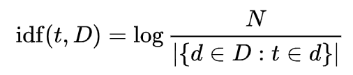
Note that only the words “for” and “sale” have a lower IDF score, since they are the only words that appear in both documents. All other words only appear in one document each, so they each receive the same score.

Next, for each document, the term frequency (tf) is calculated. This is simply a count of how often each term appears in the document. Since each advertisement only has 5 or 6 words and each word only appears once, the term frequency is never higher than 1 for each document.
With term frequency for each document, a matrix multiplication is done with the term frequencies and inverse document frequencies to arrive at the final tf-idf vector for each document.
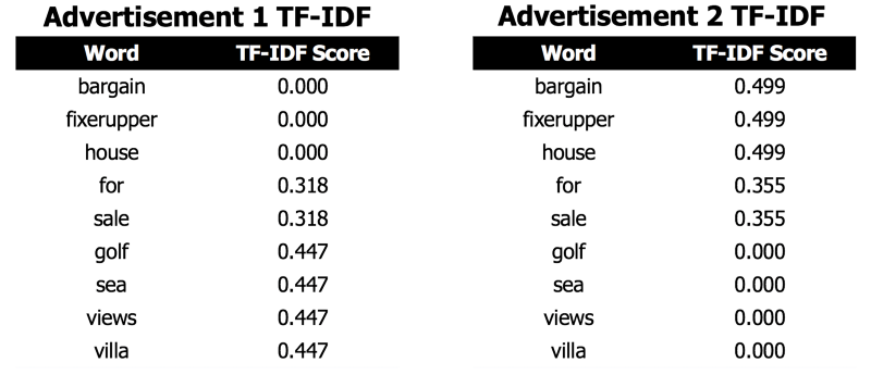
Note that the scores for the words that appear in Advertisement 2 receive a are always a bit higher than the scores for the words in Advertisement 1. Since Advertisement 2 contains fewer words than Advertisement 1, each word is counted as relatively more important.
Target variable processing
After we covered the pre-processing of the movie-descriptions, we focus now the target variable - the movie-genre.
Multi-Label
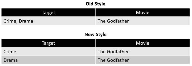
One of the most difficult questions of this project is how to deal with movies which are labelled with more than one genre. In the example of The Godfather, for instance, we see two genres, namely [Crime, Drama].
The immediate thought one could have is to label that movie as what it is, namely a [Crime, Drama] movie observation. This solution might seem appealing, given its ease of implementation, but it comes with a drawback which is illustrated below.
Considering the following three potentially possible movie-genres (a movie can have at maximum have three genre labels):
[Crime, Drama]
[Crime]
[Crime, Drama, Thriller]
Since assigning movies a genre is much less a science but rather an art, it is very difficult to say why a movie is labeled [Crime, Drama, Thriller] and not [Crime, Drama]. This potentially subjective source of labeling makes it very difficult for any Machine Learning model to learn the difference between the three examples given above.
Furthermore, we would need quite a high quantity of observation if we would like to ensure that every single potential combination of three/two movie-genres has sufficient data to train the model.
Splitting Multi-Label into Multi-Single-Label
A different solutions that seems more appealing is to split a movie observation with n-genres into n-observation, one observation for each genre. Below we find a visual explanation how this genre-splitting procedure would work:
This is then done to every movie which has more than one genre. After applying this to all observations in our dataset we end up with the following frequency distribution of genres.
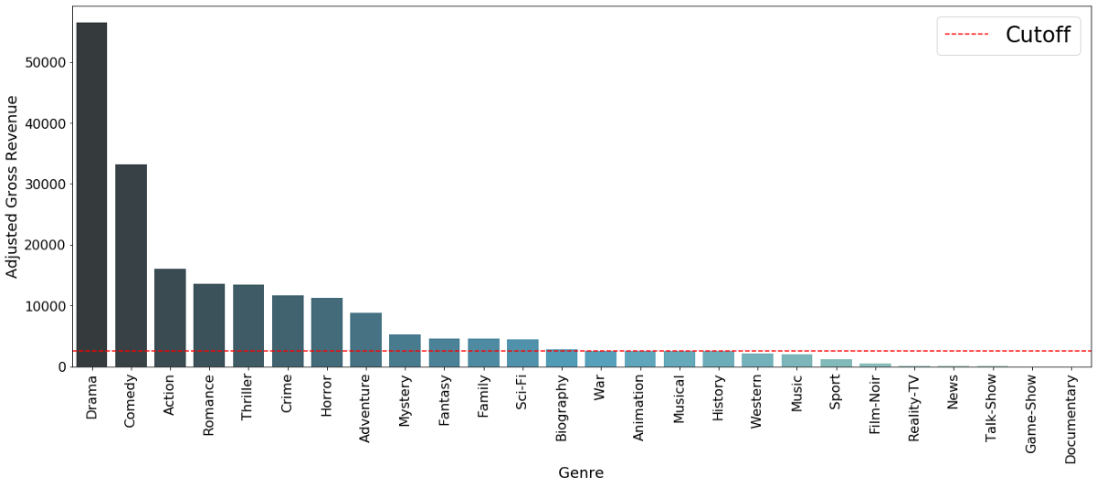
Barchart to illustrate how many single-label movie-genres we have. The cutoff is set at 2500 observationsSince this approach requires it to train a prediction model for each movie-genre individually we have to ensure a minimum number of observation for a genre in order to ensure we have enough training observations. Therefore only movie-genres with more than 2500 observations are considered, which is represented by the red cutoff line in the graph.
In the next step we talk about how we were able to help the model learn from the movie-genres.
Genre Intensity
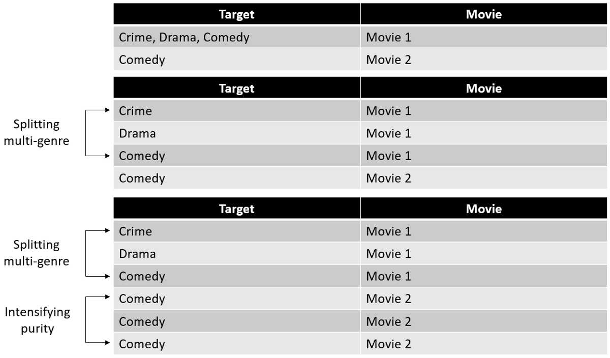
Splitting the movie in the way done above made us think about whether it is fair that a movie which is labelled as [Horror, Comedy, Thriller] carries the same weight for the prediction model for the comedy genre as the movie which is solely labeled as a [Comedy]. These two movies are probably very different pieces of art, and their descriptions are also likely to be quite different. It is reasonable to assume that the model has an easier time learning what a movie description for a [Comedy] movie looks like when seeing a “pure” [Comedy]-labeled movie description. For that reason we apply a weighting mechanism.
Namely, what is done is that a movie which is only labelled as one genre is duplicated three times, since three is the maximum amount of genres a movie can be labelled under on the ImdB website.
A movie which has three labels is not duplicated at all after the split, carrying therefore less importance for the model in contrast to a one-genre movie. A two genre-labeled movie is then duplicated once (appears 2 times) to also indicate a higher importance to the model.
Visual Example - Target Variable
A complete example of how that entire process for multi-genre problem looks like is shown below:
Model - Logistic Regression
At this point we have translated every movie description into a concise numeric vector with exactly one genre-label. When turning to the modeling side of the project, the question arises how to deal with having unbalanced multiple target variables. One solution, which is also implemented for this problem, is to train one model for each genre.
Genre Prediction
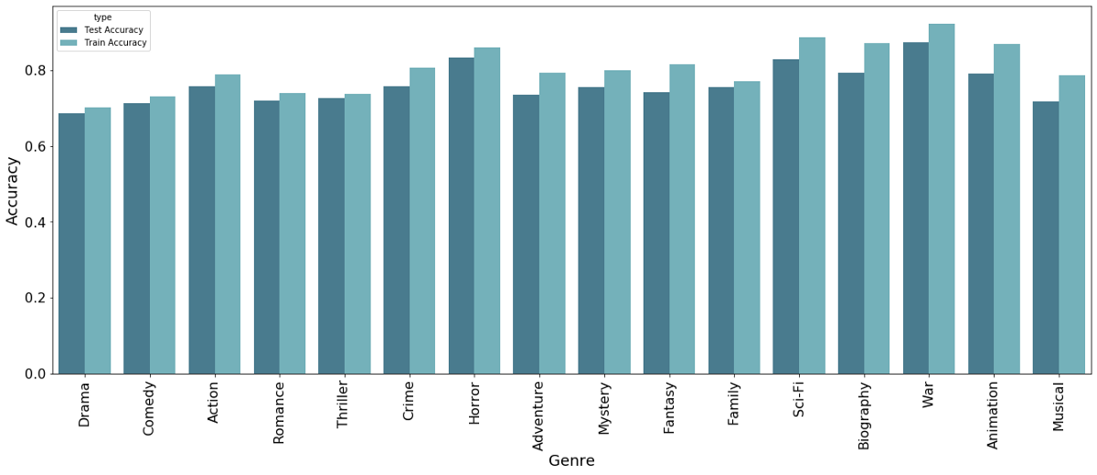
Below we see how well the different algorithms are able to predict the different genres. We can see that overall, the model struggles more to predict genres like [Drama] or [Comedy], whereas it is quite good at prediction other genres like [War] or [Horror].
The likely reason for this is the inflation of movies labeled Drama or Comedy. If you think about it, nearly every movie is a Drama in one way or another. The bar chart shown earlier also showed that the mode as well as the second most-often movie-genre is [Drama] and [Comedy]. This makes it very difficult for the model to learn these often used movie-genres.
Web App - Interactive Dashboard
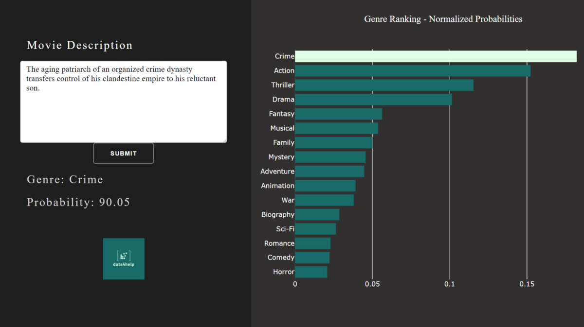
In order to present the final result of the model, we built an interactive Dashboard. Here, one can insert any real or made-up description of a plot and let the model calculate which genre it is the most likely to be.
Below we find a screenshot showing how the app interface looks. On the left side one can insert the plot and press submit. The algorithm then calculates a probability for each genre individually. All probabilities together are then normalized to sum up to one and plotted on the right side.
The genre with the highest probability is then colorfully highlighted and the shown with its individual probability on the left side.