And the Oscar goes to…

As an economist it is pretty frustrating to hear the news anchor saying that the cast of the new James Bond movies did it again. “The highest gross revenue ever…” Of course, we are more than convinced that Daniel Craig gave his everything, but the inflation rate helps as well.

Surprisingly many of monetary statistics which can be found online do not account for the phenomena of inflation. This leads to the dominance of movies produced since the 2000s, as can be seen for example here. In order to give a bit clearer view on monetary success of the different movie genres, actors and directors, this blog-post scraped data on over 300k movies from ImdB and analysed the monetary performance, while adjusting for inflation.

The blog-post is structured as follows: We start with an explanation of which deflator was used and how it was applied. Afterwards we look into the highest inflation-adjusted gross revenue by genre, stars in the movies, directors and movie titles. We conclude the post with showing the development of inflation-adjusted revenue over the years.

01 Inflation Factor

01.1 Basic understanding

There are two main terms when talking about monetary units, namely the nominal and real value of money. Nominal monetary units are the prices as they are reported at the time. When we go to the cinema today and ask for a ticket, we get told the nominal price of the ticket. If we would like to compare how much we paid for that ticket to the ticket our grandparents bought back in the day, the nominal amount they paid is not of big interest to us. It does not convey any comparable information without knowing what the price level was at that time. That is where the real value comes in - in the inflation-adjusted version of the nominal value.

In order to go from the nominal value to the real value, we need an adjustment factor for inflation. For this purpose, a price index is used. A price index gives an insight on how expensive the world is in a given time period. This is approximated by noting how expensive an extensive basket of products is for every time period. For better understanding, one could imagine going to the grocery store once every year and buying the exact same items. Afterwards, one notes what was paid for the total amount. Since the basket contains many items, it represents some sort of a diversified sample. Some things got more expensive, some things got cheaper. Overall it gives an indication what an average person has to pay to live at a certain point in time. Over the years one would observe price changes which are then said to be, on average, due to increase or decrease of the value of money. If things got more expensive, we are talking about inflation. If things got cheaper, we talk about deflation.

In reality, nobody goes to the grocery store to buy that basket. This is done on a big scale, including many more items than only the ones you can buy at a grocery store, like for example energy, transportation and water. Furthermore, effects like the substitution and quality bias also have to be considered.

The correct measures to be taken are quite complex and also not in the scope of this article and are not needed to know for the further understanding of this article.

01.2 Deflator used

Nowadays price indexes are made tailored for certain industries, in order to have a better understanding how the much cheaper/ expensive certain industries are on their own. In our case, where we are interested in comparing gross revenue of movies over the years, we used a price index for all goods instead of using one tailored to the entertainment industry. This is done to ensure a more extensive time series. Given that many movies go quite far back in time, not having a deflator for those years would make it impossible to calculate the inflation-adjusted gross revenue for those movies. We would then have had to drop all of these older movies. Since a longer time series was more important to us then a perfectly matching deflator. The time series is taken from here and plotted below.

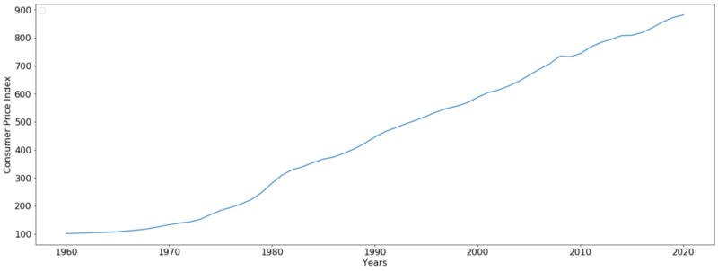
As seen above, the price index rises monotonically over the years. This means that the average price of living went up over the years, meaning we experienced inflation over the years.

Lastly we briefly elaborate of how to go from a nominal value over to a real value. As can been seen from the chart above, the base year, to which all future years are going to be compared to, is 1960. For that starting year, we see the value of 100 was assigned. This number gains meaning when comparing to the number 300 in approximately 1980. It means that the prices are 300% as high as they were in 1960. In order now to compare prices, we take the prices of 1980 and divide them by 300%, or 3. This methodology is then applied to all movie’s gross revenue.

02 Revenue figures by…

After introducing the workings of inflation and how we adjust for its effects, we now look into the more interesting results of inflation-adjusted gross revenue. This is done by splitting the results into the different variables we average by, namely Genre, Actor/Actresses (Stars) and Movie-Directors.

Before diving into the numbers, it is to be said that all number rely on the information that was provided on the ImdB website on the beginning of May 2020. That means that it could happen that newly released movies in 2020 do not have any information about the gross revenue or that some movies in especially very early years do not have any information listed regarding their gross revenue.

02.1 …Genre

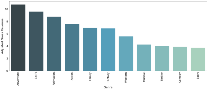
Below we can see the average inflation-adjusted gross revenue of the different genres. From today’s viewpoint, it was probably to be expected to find Adventure and Action genres on top of the list. Surprisingly, the mode (category which appeared the most often), Drama did not make it onto the top ten list. This could be potentially due to the fact that basically everything could be labelled as a Drama movie, since it does not require many special effects like for example in Adventure or Sci-Fi movies. Many of these Drama-titled movies then apparently were a financial disappointment, dragging down the average of this category.

02.2 … Stars

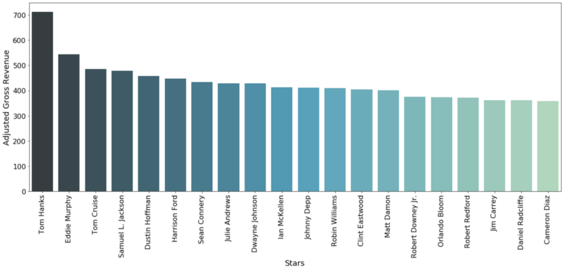
Before talking about the graphs below, some methodology of how the numbers are calculated is necessary. When encountering a movie with multiple actors (most movies), the gross revenue the movie received is then assigned to each actor with the full amount. This means that if Tom Hanks and Tom Cruise acted in a movie that brought in 100 Euro of gross revenue, the data is split in a way that both actors got assigned 100 Euro for that movie. Afterwards, the average gross revenue over all movies is calculated for each actor.

It is important to stress that this number is not the same as what the actor got paid shooting that movie. The numbers below serve as an indication to show how high the average gross revenue of a movie is when certain actors have a role in the movie.

In order to adjust for one-hit wonders, we implemented the rule that only actors which starred in at least three movies were taken into consideration.

Below we can see the surprising results of that averaging:

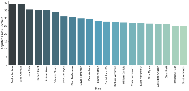
Not many people would have thought that Taylor Lautner would rank as number one on that list. Rightfully so. This statistic is a bit problematic in that it favors certain actors more than others. This theory can be explained by transferring the idea to a casino.

When asking which gambler earned on average the most money in the casino, we will not end up finding the people who go there every single day for thirty years. We will find the person who maybe went to the casino twice and won, due to luck, a considerable amount. This is because, being in the industry for a long time allows for a inevitable bad financially performing movie. Many movies of Tom Hanks at the beginning of his career for example, were not the biggest success story, even though his later movies were.

Taylor Lautner starred in exactly four movies in our dataset. He probably acted in more, but there are four movies under the ImdB link given above, for which Taylor Lautner was listed as an actor. These movies are:

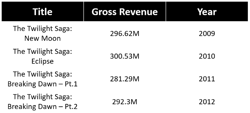
The question may arise why Robert Pattinson or Kristan Stewart are not listed in the average top ten list, even though their co-star Taylor Lautner is. The answer is the number of movies shoot for the former two actors. Robert P. and Kristan S. both starred in many more movies than only these four and therefore have a lower average. This example shows how this graph above gives a biased view.

If, on the other hand, we would like to see which actor/actress ranks highest when using cumulative gross revenue over all movies they starred in, we find a more expect-able result, with Tom Hanks as number one.

02.3 … Directors

The same problem we encountered with the actors/actresses above rears its head again when ranking movie directors by average revenue. Looking at the graph below, one might wonder why the household name Steven Spielberg only ranks so low on this results table.

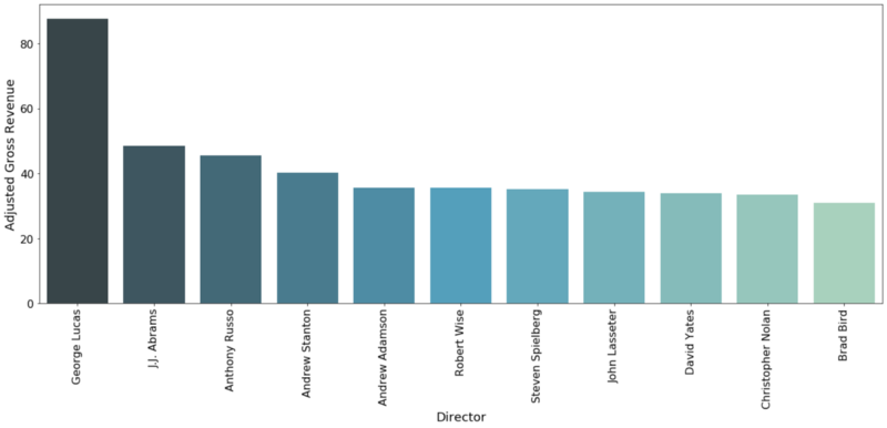
The answer is again the lucky observations which did not encounter a flop during their career, but also did not shoot as many movies as some of the others. When looking again at the cumulative statistics, it becomes clear who rules this business.

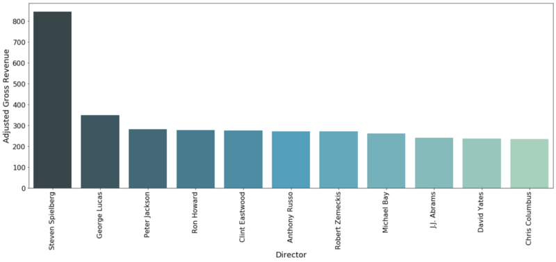
The cumulative inflation-adjusted gross revenue for Steven Spielberg is now twice as high as the one for George Lucas.

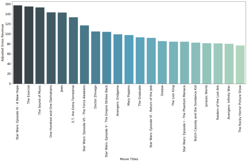
02.4 …by movie

Maybe the most interesting graph of this post is the one below. Here we show the inflation-adjusted gross revenue of all movies since 1960. The winner is Star Wars IV - A New Hope released in 1977. Even though Avengers: Endgame got a lot of publicity lately given its massive gross revenue, it’s still smaller than One Hundred and One Dalmatians. We are aware that the ranking shown below differs somewhat to other rankings shown on the web, even to ones which adjust for inflation. This could have many reasons, ranging from different sources for the gross revenue over to using a different price index.

03 Development by Genre

Lastly it would be interesting to see how the inflation-adjusted gross revenue changed over the years. For this purpose two graphs are shown below, one for all years in the data and another one which has a focus on the 2000s.

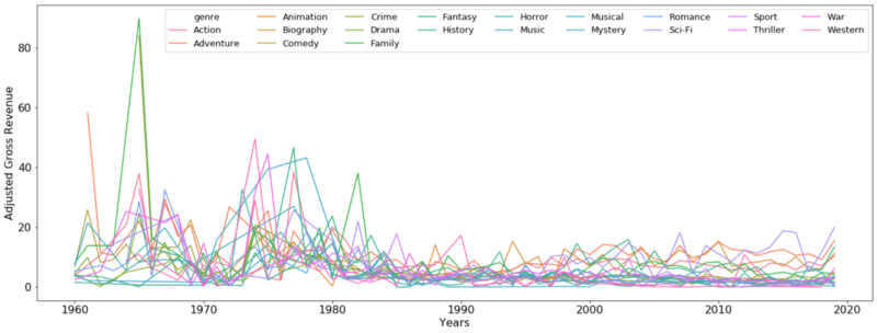
03.1 Overall

In order for the statistic not to be completely distorted by stark outliers, only years are considered which have more than one movie in a certain year.

Especially interesting is the performance of the Family genre, which spiked around the 1960s and continued strong until this day. From a financial perspective the strong performance of family movies is not surprising, targeting a market which pure action movies cannot take.

It is also visible that the inflation-adjusted gross revenue average was considerably higher in the early years of the data compared to the more recent years. That fact can also explained by the fact that there are considerably more movies produced in the last twenty years in contrast to the years between 1960–1980. The increase of movies produced is, according to the data, not completely aligned with people going to watch these movies. This fact leads to a lower average of gross revenue nowadays.

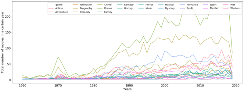
To prove this theory outlined above is proven below. The two graphs below show the cumulative inflation-adjusted revenue over the years as well as the number of movies in every year since 1960.

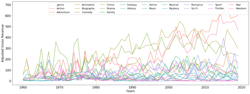
It is clearly visible that nowadays there are massively more movies produced and the industry as a whole got consistently larger over the years. On average, though, each movie had a smaller gross revenue given the sheer amount of movies and competition.

The increasing number of feature films made in a year is not the only thing impacting declining revenue per film. The number of other entertainment options available to people have also increased substantially, with streaming services today, and movie rentals available from about the 1980s onwards. These factors all likely influence the much higher adjusted revenue per movie for movies made in the 1960s and ’70s.

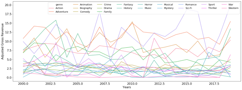
03.2 Focus on 2000s

As a last step, we thought it would be interesting to zoom in to the average inflation-adjusted gross revenue since 2000. When comparing the average inflation-adjusted gross revenue in last years, we find a very volatile line for the Sci-Fi and Adventure category. This is likely do be due to the blockbuster releases in these years.

We would like to end up on the nice note that the graph below shows that the exploding-cars-showing Action genre is still behind the more thoughtful and happier Family genre.

04 Next up

The next blog post looks more into the movie description and makes an attempt to predict the movie category using only the description text of a movie.