Empirical Evidence to common Stock Portfolio Questions

An intuitive and replicable explanation to some of the most important questions of portfolio building

At first glance investing seems like rocket science to many people. The sheer amount of possible assets to invest in and the amount of fancy sounding finance terms might seem intimidating. This blog-post elaborates on three of the most asked questions when building a portfolio. This is done by starting with a theoretical explanation and, more importantly, an empirical validation using Python.

We start by loading all the relevant packages and putting the directories for our project in place.

# Packages
import pandas as pd
import numpy as np
import os
import matplotlib.pyplot as plt
from tqdm import tqdm
# Paths
main_path = r"/Users/paulmora/Documents/projects/markowitz"
raw_path = r"{}/00 Raw".format(main_path)
code_path = r"{}/01 Code".format(main_path)
data_path = r"{}/02 Data".format(main_path)
output_path = r"{}/03 Output".format(main_path)

Loading asset returns

In order to make the financial theory come alive, we need to create financial return time-series data. In order to work with real financial returns, we use the yahoo finance API. This is done by using the pandas webreader. This powerful package can, among others, download historical price data for different stock tickers. A stock ticker is the abbreviation of a company name used at the stock exchange. For example, the ticker-name of Apple is AAPL. An extensive list of companies and their stock tickers can be found here.

After downloading the aforementioned excel, we upload them into Python with the following lines.

# Loading the tickers
ticker_excel = pd.read_excel("{}/ticker.xlsx".format(raw_path))
ticker_list = list(ticker_excel.loc[3:, "Yahoo Stock Tickers"])

Now it is time to build a function with which we can create financial returns for a certain number of assets. As the input parameters we select the number of return time-series we would like and for how many years back from today we would like them. The following function allows us exactly that.

def financial_dataframe_creation(ticker_list,
                                 number_of_stocks,
                                 starting_year):
    """
    This function imports finanial price data from yahoo from a
    pre-defined list of stock-tickers.
Parameters
    ----------
    ticker_list : list
        list with stock-tickers used by yahoo finance
    number_of_stocks : int
        number of stocks desired in the final dataframe
    starting_year : TYPE
        year from which we would like to extract financial data from
Returns
    -------
    returns : dataframe
        this dataframe contains daily returns for as many
        stocks as were specified in the beginning
"""
df_prices = pd.DataFrame()
    i = 0
    while len(df_prices.columns) != number_of_stocks:
        ticker = ticker_list[i]
        try:
            tmp = web.DataReader(ticker, "yahoo",
                                 "1/1/{}".format(starting_year),
                                 dt.date.today())
            df_prices.loc[:, ticker] = tmp['Adj Close']
        except KeyError:
            pass
        except RemoteDataError:
            pass
        i += 1
    returns = np.log(df_prices / df_prices.shift(1)) * 252
return returns

Before tackling any question we go for a test-run of the function to see whether it returns the desired output. The following code:

min_year_restriction = 2010
number_of_stocks = 5
returns = financial_dataframe_creation(ticker_list,
                                       number_of_stocks,
                                       min_year_restriction)

results in this output:

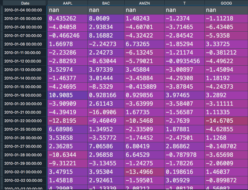
We can see that the different assets are now displayed as columns names and we find one annualized return information for every day of our time series. With the knowledge that our function works, we can start to answer the questions.

“The more stocks in the portfolio the lower the overall risk”

Theory

This statement might seem counter-intuitive at first glance. Having more stocks in your portfolio might seem that there are more things that could go wrong. The reason that this is not the case is related to a concept called diversification.

Imagine that you only have one stock in your portfolio. In that scenario your portfolio is predominately exposed to two kind of risks: Market risks and firm-specific risks.

The firm-specific risks are specific to one individual firm. These risks range from a sudden death of the CEO (assumed to be negative news) up to unexpectedly finding oil on the company’s grounds (assumed to be positive news). Note that if an investor is only carrying one stock in their portfolio, they are heavily exposed to these company-specific risks.

Market risks compromises risk that affect macroeconomic factors like interest rate changes, inflation, unemployment, and so on. If for example the global economy enters a recession and overall fewer goods are sold and bought, the one individual firm in the investor’s portfolio is also going to be affected by it.

When now investing not in one, but in multiple stocks, the company specific risk reduces quite massively given its small contribution to the overall portfolio performance. The market risks on the other hand, given its wide-reaching and all-affecting implications, has an impact on the total portfolio performance nevertheless. Since market risks affect all stocks, they are also referred to as systematic risk. This kind of risk does not reduces when we increase the number of stocks within our portfolio.

Empirical Evidence

In order to validate the financial theory outlined above we create multiple portfolios with an increasing amount of stocks in each portfolio and re-calculate the risk of each.

We start by initializing time series data for 500 stocks, starting in the beginning of 2016 up until today. This is done using the following code

min_year_restriction = 2016
number_of_stocks = 500
returns = financial_dataframe_creation(ticker_list,
                                       number_of_stocks,
                                       min_year_restriction)

Now we would like to show how the overall portfolio risk reduces when we include more assets in our portfolio. For that we calculate and store the portfolio risk of a given portfolio of the first 25 assets. Afterwards we add further 25 assets to that portfolio and re-calculate the risk again and so on. This is done through the following code:

step_size = 25
risk_list = []
num_stocks_list = []
for num_stocks in tqdm(range(1, number_of_stocks+2, step_size)):
    portfolio = returns.iloc[:, :num_stocks].copy()
    num_of_companies = len(portfolio.columns)
    cov_matrix = portfolio.cov()
    sum_covariances = cov_matrix.sum().sum()
    weighting = num_of_companies**2
    portfolio_variance = sum_covariances / weighting
    risk = np.sqrt(portfolio_variance)
    risk_list.append(risk)
    num_stocks_list.append(num_of_companies)

When plotting the results we get the following picture:

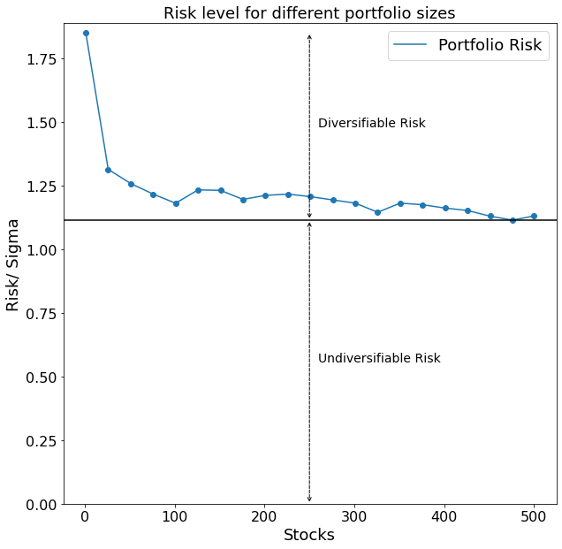
Our hypothesized reduction in overall portfolio risk with an increasing amount of stocks shows up nicely. The black horizontal line drawn in the graph furthermore depicts the level of risk of a portfolio which cannot be further reduced even when including more stocks into the portfolio. That is because all stocks are going to be affected by the volatility of the market as a whole. This minimum threshold of risk is also called undiversifiable risk, whereas we call the risk which is possible to reduce the diversifiable risk.

“The important risk kind of an asset is its covariance with other assets and not its own volatility”

Theory

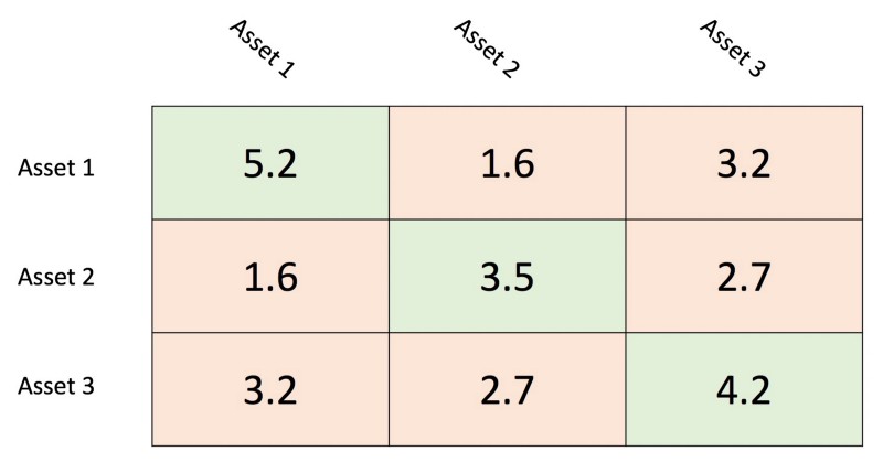
The answer to the question of how to calculate the risk of an equity portfolio is easier than one might initially think. It is actually only the sum of the portfolio covariance matrix. The covariance matrix shows each asset’s variance on the diagonal and the covariance with each other asset in the upper and lower diagonal matrix. As an example let us consider the covariance matrix below. The variance are denoted by a light-green shaded background whereas the covariance have a light-red shaded background. It is important to note that the upper diagonal matrix and lower diagonal matrix are identical. That is because the covariance of A and B is equal to the covariance of B and A.

It is important to know how the number of variances and covariance scale with the size of the portfolio. A portfolio with n-assets for example has exactly n variances and n²-n covariances. It is easy to see that with a higher number of n the covariances outnumber the variances significantly.

Empirical Evidence

To check whether that is also empirically the case, we implement the following code.

step_size = 10
maximum_number_of_stocks = 100
list_num_stocks, sum_variances, sum_covariances = [], [], []
for num_stocks in range(1, maximum_number_of_stocks+1, step_size):
    portfolio = returns.iloc[:, :num_stocks]
    covariance_matrix = portfolio.cov()
    list_num_stocks.append(num_stocks)
    variance_returns = np.nansum(np.diag(covariance_matrix))
    sum_variances.append(variance_returns)
    sum_covariances.append(covariance_matrix.sum().sum()
                           - variance_returns)

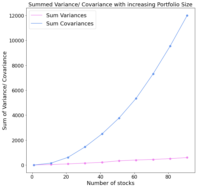
The plot above shows us exactly the hypothesized outcome. The over sum of covariances represents a multifold of the sum of variances of the portfolio. This finding entails interesting implications for the selection process of an asset. The asset’s own variance carries little to no importance for the risk of a well-diversified portfolio.

“A longer investment horizon reduces the portfolio risk”

Theory

The investment horizon describes how an investor plans to hold the portfolio. These ranges can span from merely a few days up to multiple years. When deciding for a longer investment horizon an investor typically allocates most of their assets to a higher risk area, like equities. This is because the larger price swings, equities exhibit in the short term, have no impact on the long-term goals of the investor.

Empirical Evidence

The following code shows how we can empirically test this theory.

number_of_stocks = 100
weighting = 1/(number_of_stocks ** 2)
years = np.arange(2000, 2020, 2)
risk_list = []
for year in tqdm(years):
    time_returns = financial_dataframe_creation(ticker_list,
                                                number_of_stocks,
                                                year)
    portfolio_var = weighting * time_returns.cov().sum().sum()
    portfolio_std = np.sqrt(portfolio_var)
    risk_list.append(portfolio_std)

The code above first takes 100 arbitrary stocks using our function which we declared in the beginning of this post. Afterwards the portfolio variance for an equally weighted portfolio is calculated for different time-spans. The result is the following plot.

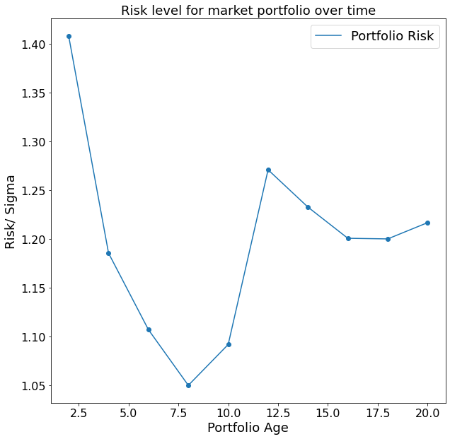
Interestingly, even though we can see an overall trend to a smaller risk level over time, the relationship is not perfectly negative. This is because we find a local minimum after around eight years. This finding is likely to be explained by the financial crisis 2008. Given that we started to track our portfolio performance in the year 2000, after eight years we find our portfolio in one of the most financially unstable times in modern history. After a couple of turbulent years, we find the portfolio risk to decrease again, which is quite an affirmative sign in the direction of our hypothesis that a longer time horizon reduces our portfolio risk.