Outlier detection in Real Estate Data

Preparing the data for feature extraction and modeling In the prior post, we outlined how we scraped real estate data for 42,367 properties in Spain. Before jumping directly to any modeling exercises, it is important to look at the variables at hand. Data inspection is essential in order to see whether the set goal is actually achievable with the given data, and how we can improve the data quality. This section is structured as follows:

1. Assessing the data
2. Why are outliers problematic?
3. Identifying outliers
4. Defining the cutoff level
5. Conclusion

01 Assessing the data

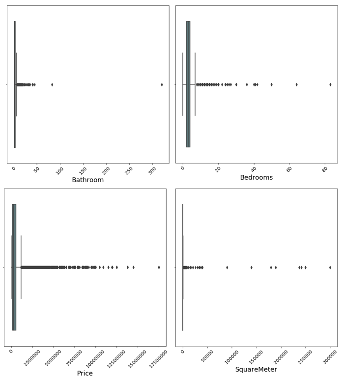
In order to get a first feeling for the data, it is always wise to plot the variables. Below we see boxplots of the four main variables. The variables are the number of bedrooms, number of bathrooms, number of square meters and the price of the property.

It is clearly visible that all variables are heavily skewed to the right. That means that most of the data is centered at the left side of the distribution, with fewer observations on the right side. This occurs because of two reasons: the first is that all four variables are capped at zero on the lower side. This leaves less room for outliers on that end of the distribution. Secondly, even though the website is supposed to show only valid houses and estates, there are still some properties which are not valid and skew the distribution drastically to the right, like large commercial properties such as hotels and restaurant spaces.

We can see from the graph above that there are apparently several observations with more than 50,000 square meters or over 300 bathrooms. These are definitely not features one would expect to see in an ordinary house - the validity of these observations should be questioned.

It would be easy to simply drop any observation with a insensibly high or low amount of a certain variable, but there are major problems with doing so. The first problem is how to define what is a too high or low amount. Choosing an arbitrary amount is not scientific and hard to defend in front of the project owner. The following section outlines other more scientific methods for defining what makes an outlier.

02 Why are outliers problematic

In regression estimation problems, outliers can influence the algorithm massively and distort the results and predictive power of the model. Consider a multiple linear regression: each beta coefficient tries to quantify a linear relationship between the respective feature and the dependent variable. Introducing an extremely high or low observation strongly influences this linear relationship and distorts it. That is because of the loss function the algorithm tries to minimize, which in the case of multiple linear regression it is the mean squared error (MSE). In order to minimize the loss, the algorithm tries to fit better to the outlier given the enormously large error the outlier produces.

This problem also holds for other models such as Boosting and Bagging models. A common misconception is that bagging models, such as Random Forest, are insensitive to outliers because of their non-parametric nature. This is not true, especially not when you have more than one outlier. The reason for that is, again, the loss function. Like in multiple linear regression, the bagging model overfits to the outliers and finds an overall worse performing result compared to a model which does not contain outliers at all.

The problem of outlier(s) with boosting models is even greater. Boosting model such as AdaBoost and Gradient Boosting are iterative models, meaning that in contrast to bagging models, the algorithm fits a first model, sees where it performs relatively badly, and will puts more emphasis on those observations in the later iterations. Outlier(s) make this task much harder - the model then builds itself primarily on a few non-sensical outlier observations.

02.2 Why dropping outliers is problematic

Generally it should be said the simply dropping outliers to improve the model at hand should not be taken lightly. Simply dropping observations to improve the model at hand is a form of data manipulation and is not justifiable scientifically or statistically.

Removing outliers could potentially lead to a biased sample. Furthermore, it could also make the results of the predicting algorithm completely meaningless as the results would not apply to any prospectively definable population. Looking in the advertisement texts of properties with more than 300 bathrooms or 50,000 square meters reveals that these observations are often commercial land properties or even multiple houses bundled together. Given the nature of this project, namely building a prediction model for house prices in Spain, it is valid to drop observations which do not fall in the category of a residential property.

03 Identifying outliers

When it comes to identifying outliers, there are many methods which can be useful. This post uses three of the most common ones, namely the percentile method, the interquartile range method and the empirical rule. It is important to stress that there is no holy grail in outlier detection and different models will result in different conclusions. In order to make a well-rounded decision and not to rely too much on any method, we made the decision to classify an observation as an outlier only if all three methods classify it as an outlier. In the following sections all methods are explained and the implementation of the method in code is shown.

03.1 Percentile based Method

The percentile method cuts off a predefined percentage amount from the top and the bottom of a distribution (if both sides are desired). In order not to cut off too much of the observation, a cutoff value of 1% is commonly used. That means that the top and bottom 1% of the a variable is labelled as an outlier.

def pct_method(data, level):
    # Upper and lower limits by percentiles
    upper = np.percentile(data, 100 - level)
    lower = np.percentile(data, level)
    # Returning the upper and lower limits
    return [lower, upper]

03.2 Interquartile Range Method

The interquartile range approach first calculates the interquartile range (IQR) of the data. The IQR is defined as the difference between the 75 and 25 percentile of a variable. This IQR is then multiplied with 1.5. Any data that is then further away than the 75 percentile plus 1.5IQR or 25 percentile minus 1.5IQR is classified as an outlier.

def iqr_method(data):
    # Calculating the IQR
    perc_75 = np.percentile(data, 75)
    perc_25 = np.percentile(data, 25)
    iqr_range = perc_75 - perc_25
    # Obtaining the lower and upper bound
    iqr_upper = perc_75 + 1.5 * iqr_range
    iqr_lower = perc_25 - 1.5 * iqr_range
    # Returning the upper and lower limits
    return [iqr_lower, iqr_upper]

03.3 Standard Deviation Method (Empirical Rule)

The standard deviation approach arises from the so called empirical rule which states that given a normally distributed variable, approximately 99.7% of the data is within three standard deviations. This approach then classifies any observation which is more than three standard deviation below or above the mean as an outlier. It is essential to note though that this approach only works if the data is approximately Gaussian.

def std_method(data):
    # Creating three standard deviations away boundaries
    std = np.std(data)
    upper_3std = np.mean(data) + 3 * std
    lower_3std = np.mean(data) - 3 * std
    # Returning the upper and lower limits
    return [lower_3std, upper_3std]

03.4 Combination of all three methods

As mentioned earlier, dropping outliers should only be done in extreme cases and when the observation are clearly misrepresenting the project task. For that reason we only classify an observation as an outlier if it satisfies all three conditions introduced above. Combining all three approaches is done in the following way:

def outlier_bool(data, level=1, continuous=False, log=False):
    # Taking logs is specified
    if log is True:
        data = np.log(data + 1)
    # Obtaining the ranges
    pct_range = pct_method(data, level)
    iqr_range = iqr_method(data)
    std_range = std_method(data)
if continuous is False:
        # Setting the lower limit fixed for discrete variables
        low_limit = np.min(data)
        high_limit = np.max([pct_range[1],
                             iqr_range[1],
                             std_range[1]])
elif continuous is True:
        low_limit = np.min([pct_range[0],
                            iqr_range[0],
                            std_range[0]])
        high_limit = np.max([pct_range[1],
                             iqr_range[1],
                             std_range[1]])
# Restrict the data with the minimum and maximum
    outlier = data.between(low_limit, high_limit)
# Return boolean
    return outlier

Two options are important to note within this function. The first is that for variables which are continuous, we also take a look at observations with obscurely low levels. This is done since several properties report a number of square meters of 1. These observations are spam ads, which clearly do not belong in the data. For discrete data (number of bedrooms or bathrooms) we only use the minimum value of the data series.

The second important argument is the use of logs. Given the high skewness of our variables, using the outlier detection methods has several issues. Firstly, the empirical rule does not work since it requires an approximate Gaussian distribution. Secondly, given that the goal is to remove as few outliers as possible, squishing extreme values closer to the rest of the data gives them a better chance not to be identified as an outlier in the first place.

Given the reasons outlined in the paragraph above, all variables are log-transformed before the outlier detection methods are applied.

04 The cutoff levels

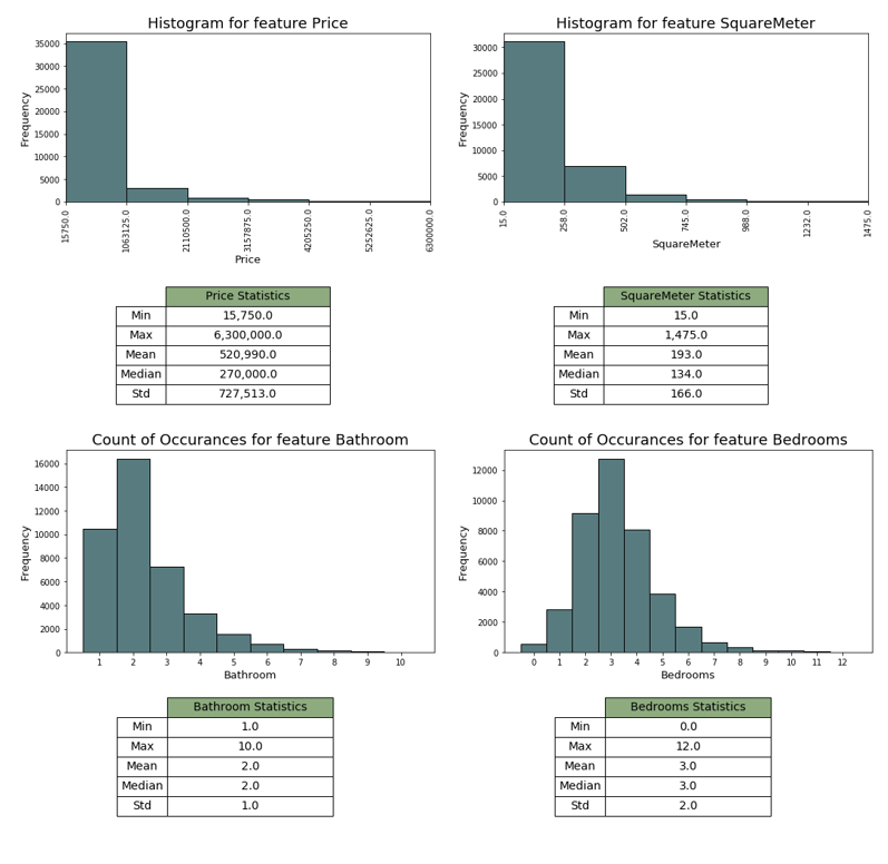
This section gives an indication as to how many observations were thrown out and where the cutoff variable was set for all four variables. The table below shows the cutoffs for each variable as well as there respective minimum and maximum.

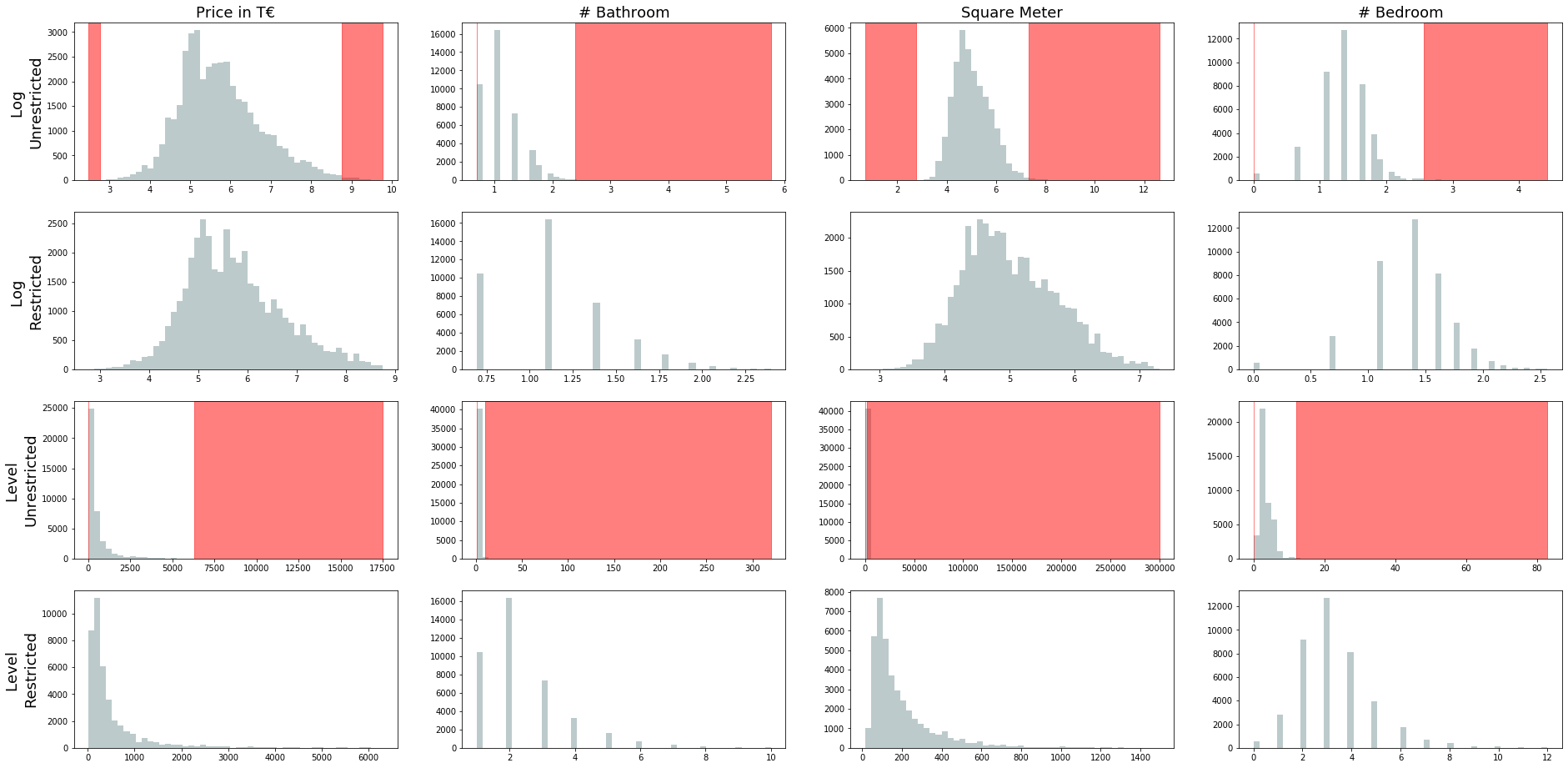
All cutoff level seem sensible. The cutoffs allow easily for all kinds of properties, but also allow for multi-million mansions priced up to €6,300,000. In order to have a better visual understanding of how exactly the outliers have been cut, the graph below should shed some light. The first row of the graph below shows the log values all four variables, before removing any observations (unrestricted version). The red area then shows what our above defined, three methods using, outlier detection model regarded as an outlier. The second row then shows the distribution of the log values after the outliers have been removed (restricted version). The third row then shows the non-transformed data unrestricted and with a red indication shown where the cutoff happened. The last row then shows the restricted version of the raw values.

For all variables we can see a clear reduction in skewness and something which come closer to a Gaussian compared to the unrestricted model. Looking at the summary statistics below, we can also see that the skewness is still there but much less rightly skewed than before. Going forward, there might still be a case of applying logs on the variables in order to dampen the higher values within the price and square meter variable.

05 Conclusion

At the end of this post, it is important to remind ourselves where we came from and why removing outliers is an important step before moving on to modeling and prediction. After scrapping around 40k properties, we took a first look into the data. We found that the data is heavily affected by some extreme observations that do not represent residential properties. We then outlined potential problems of keeping and dropping outliers and decided to only remove observations that represent truly obscure cases. The next step is to try to make sense of the dataset we have now that outliers have been removed. More specifically, the next post will apply some clustering in order to separate estates by their variable characteristics.