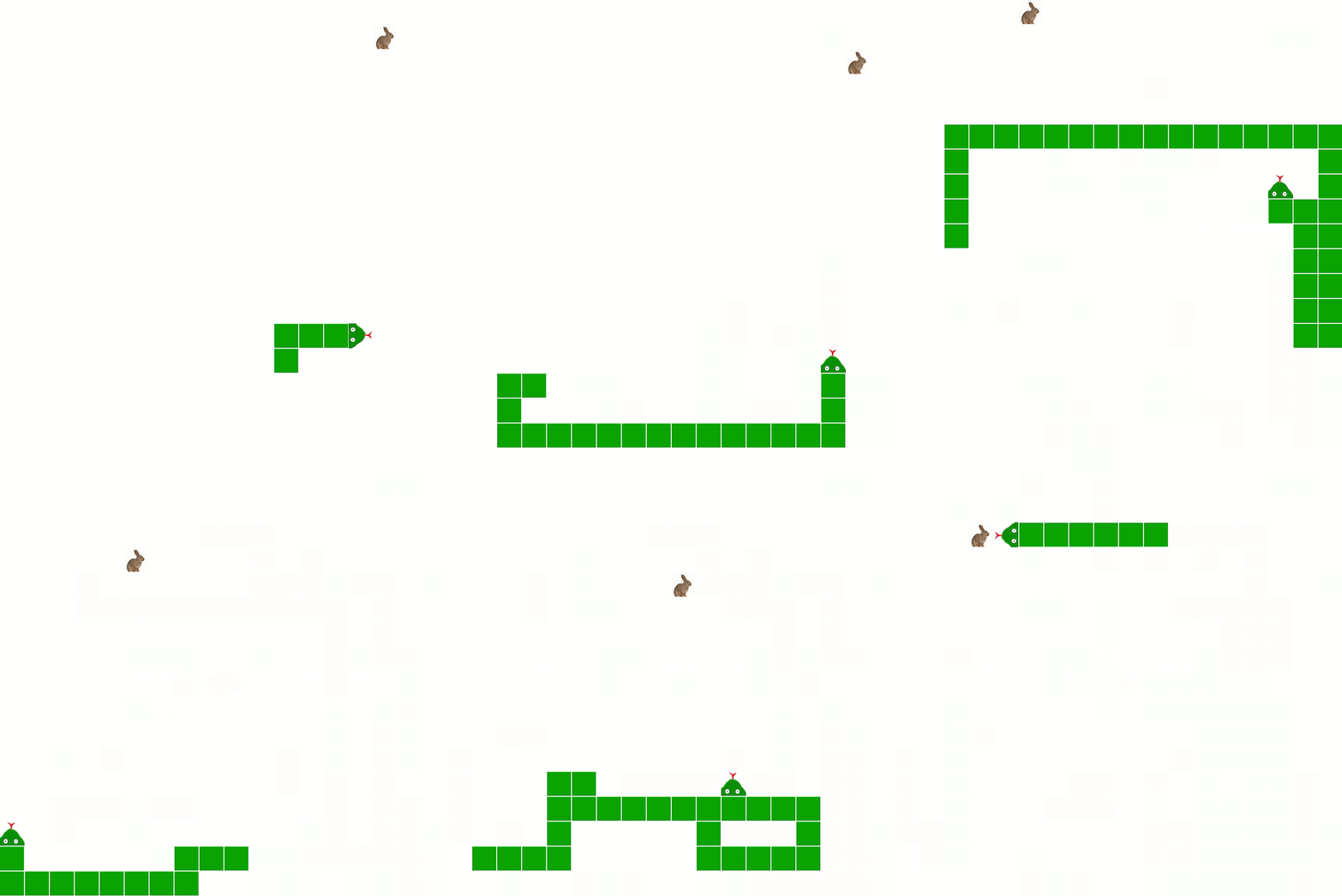
Human vs. Machine — Reinforcement Learning in the Context of Snake
This blogpost elaborates on how to implement a reinforcement algorithm, which not only masters the game “Snake”, it even outperforms any human in a game with two players in one playing field.
Reinforcement Learning: Basics of Q Tables
For the Snake to play the game itself, the Snake has to answer at every step the very same question: What to do when faced with conditions such as a certain position of its body, position of the snack and position of the walls which would end the game if touched by the Snake. The information used to describe the situation or state of the Snake is referred to as “state variables”. A visual example is made to illustrate the problem at hand in a different context. Imagine a fictional character who is dressed in one of the following four ways:

The way the character is dressed should be taken as a given and represents the state variables. Furthermore, the fictional character now has four possible destinations to go to next. The destinations look like this:

The question at hand is: at which of these four places would the fictional character experience the most pleasure, given its clothes? Answering this question might seem intuitive. Perhaps this experience of wearing too warm clothing (or even winter clothing) in a warm environment has already been made in the past, and the lesson from the discomfort experienced as a result has been learned. Furthermore, this combination of state variable and action has also already been evaluated. In the situation of winter clothes and the beach, the evaluated outcome was most definitely negative. This evaluation of an action given its state variable that we have experienced and learned from in our own pasts is exactly the point of reinforcement learning. Using past experiences to indicate whether a certain action is a good or bad decision is exactly how Q-Tables work in the context of reinforcement learning. It is crucial to notice that a certain action given the state was only possible because the situation of wearing winter clothes (state variables) and going to the beach (action) were already experienced.
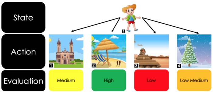
Using logic of how it should theoretically feel to wear warm clothes at the beach without having prior experience is an inference and would require some sort of forecasting model, which is not used in the basic setting of Q-Tables. This implies that when a situation occurs where the fictional character is dressed in a way that it had never been before, meaning it is not known how pleasurable it would be to go to one of the four possible locations dressed in that manner. The image illustrates this last argument, meaning that it has to visit all four different locations at least once to make an evaluation.
Q-Tables applied in the game Snake
The difference between the situation of the fictional character and the Snake is how the state is described and what kind of actions are at hand. The image below shows a normal scenario of a Snake game. The Snake’s body is shown as purple, the boundaries of the playing field are black, and the objective (the snack) is shown as green. The Snake has now four options what to do: it could go left, right, up or down. In the following situation it might seem intuitive for the Snake to go right and simply eat the snack. Why is that intuitive? Because this action was taken in the past and received as a positive experience. What about going left and backing up into itself? This combination of state and action was experienced as something negative.
As visible on the right side, the state at hand is described by two kind of variable categories. The “Danger Variables” give an indication whether the Snake is of risk of dying when going into a certain direction. As discussed before, going left and backing up into itself would kill the Snake. The other variable category is related to the snack the Snake would like to eat. This snack lies in a 90-degree position away from the Snake’s head and is only one field away to be eaten.
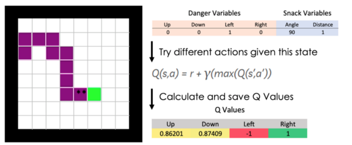
A examplatory position of the snake and the calculation of the Q-Value
Foundations of the Bellman Equation
In order to understand the magic of Reinforcement learning, it is necessary to discuss the Bellman Equation which is stated on the right side of the graphic. This equation calculates the Q-Values for every move the Snake can take. In order to understand what a Q-Value is, it is necessary to introduce the concept of rewards and penalties. Within Reinforcement Learning the algorithm receives feedback immediately for every action it takes. In the case the algorithm did something favourable (going to the beach when dressed in summer clothing), then a positive reward of is noted. Following the same logic, a negative reward is given for something unfavourable (going out into the snow with summer clothing) and a neutral reward is given for action which did not lead to a success or failure of the algorithm (going to church in summer clothing). For scaling purposes, normally a standardized reward structure is taken. This means for our Snake example: In case the Snake eats the snack, the algorithm receives a reward of plus one, if it dies it receives a reward of negative one and if it simply makes a move without dying nor eating a snack, it receives a reward of zero. This reward is represented by the “r” within the Bellman equation.
Moreover, it is important for the algorithm to apply some sort of forward thinking. As for many games or tasks, it is not only important to receive the next immediate reward, but also to consider the longer-term goal after that. This consideration of the importance of the future is denoted and incorporated by the “γ”. This gamma coefficient should be carefully chosen. If it is too low, then the agent will not care about the future and only try to receive the reward of the current state as soon as possible, sacrificing a favourable position for the long-term reward to come. If the discount rate is chosen too high, then the current goal is neglected since it carries a relatively low importance compared to the future. The max Operator within the Bellman Equation can be interpreted as the calculated upcoming rewards when a certain action is taken, meaning that if the Snake decides to go left then it knows that it will go e.g. right afterwards to receive the snack. Hence, not only the “left movement” carries importance, but also the upcoming “right movement”.
Q Table Performance
When the Q-Table is completely filled out, it is nothing other than a lookup table for the algorithm to decide what to do when a certain state occurs.

The Q-Table serves as a simple lookup table which is iteratively filled as soon as a certain state is shown to the algorithm
The next question would then be, how does the algorithm fill the table? The answer is simple, it just starts collecting the data itself by moving at random. By moving at random the algorithm collects its own data and iteratively gets better and learns how to react in every observed state. Since the algorithm is constantly learning, it is more and more encouraged to apply actions it learned in the past. Below two graphics are visible. On the left, the untrained algorithm is shown. It is clearly visible that there is no clear pattern in its movements and it strikingly fails to succeed in the game. On the right, on the other hand, a trained algorithm is shown. This difference is that this algorithm has learned to make its own decisions after approximately 50.000 iterations.
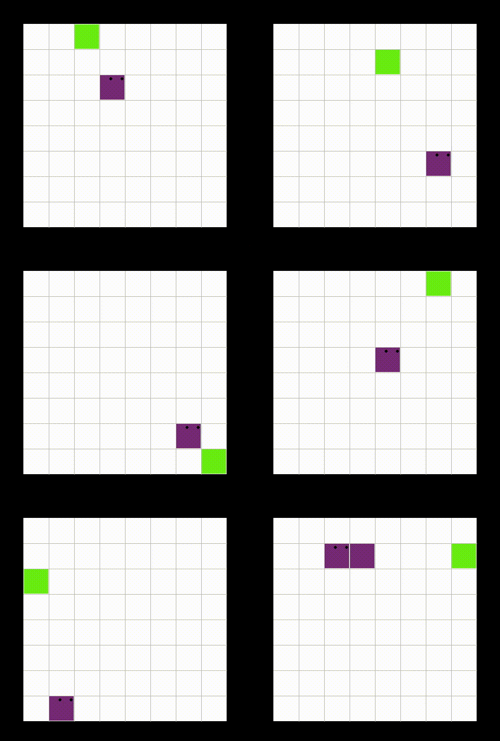
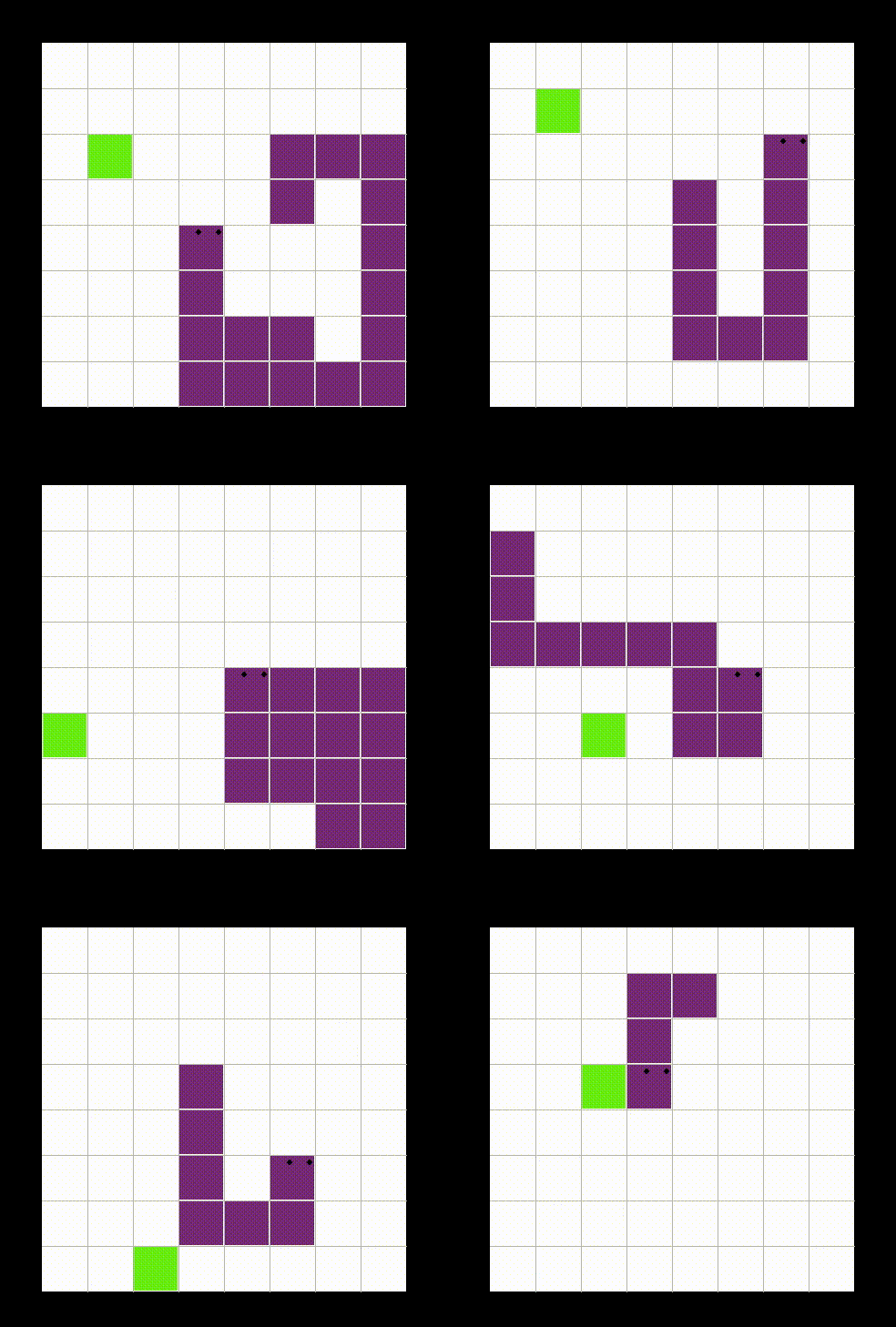
On the top an untrained algorithm is shown. It moves via random actions taken. On the bottom an algorithm which was trained with approx. 500k iterations is shown. It performs fairly well already.
Every time the Snake dies, the Snake is less advised to use a random algorithm for decision making purposes, but rather to make the decision given its past acquired knowledge. This approach is called Epsilon Decay, but there are other ways to steer the exploration and exploitation problem faced. A summary of the most well-known approaches is given below:
Epsilon Decay: The algorithm is taking a random action with probability epsilon. This probability then decays with a predefined rate before the next action is taken
Upper Confidence Bound: The action with the highest uncertainty is taken. When an action is taken often enough, and the outcome of that action is less uncertain, another action is taken
Epsilon Greedy: A random movement is taken with a pre-defined probability, in comparison to the Epsilon Decay approach, this probability never changes, meaning that even a trained model still takes random action.
When training the algorithm, the graphic that everybody would like to see is how the average reward develops over time. An increase in this chart would imply that there is a positive correlation between the numbers of games the algorithm saw and how well the algorithm succeeds. The chart below shows exactly the desired pattern: Over time the Snake algorithm increases its average body length. Since creating a longer Snake is the goal of the game in the first place, the algorithms trains!
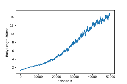
Moving average (300 units) of the body length of the Snake over 50k training steps
Introducing a second player
Lastly, the game is made to appeal more to the end user. For that purpose, a second, human-controlled player (snake) is inserted in the very same playing field where the algorithm is already playing. Furthermore, the visual appearance of the now two Snakes is enhanced. This enhancement required only some simple editing in MS Paint.
No changes had to be made to the machine-controlled Snake. Whenever it faces the human controlled Snake, it will simply treat it as it treats any danger proximities- it avoids them! Because of the incredibly fast reaction time of the algorithm, no human stands a chance (even after playing 50 times, no one came close to beating it).
Everybody is encouraged to try to beat the machine. The rules are simple: you have one minute to score a higher Snacks-eaten/Deaths ratio than the machine. The entire code is found here on Github.
