Richter’s Predictor- Data Challenge from DrivenData

Scoring in the top one percent in the Richter’s Predictor: Modeling Earthquake Damage on DrivenData.

Next to Kaggle there are many other websites which host highly relevant and competitive data science competitions. DrivenData is one of these websites. The main difference between the renowned Kaggle and DrivenData is probably the topics of the challenges. Wheras Kaggle hosts more commercially driven competitions, DrivenData focuses more on philanthropic topics.

We, data4help, took part in one of their competitions and scored out of around 3000 competitors in the top one percent. This blogpost explains our approach to the problem and our key learnings.

01 Introduction - Problem Description

The project we chose is called Richter’s Predictor: Modeling Earthquake Damage. As the name suggests, the project involves predicting earthquake damages, specifically damage from the Gorkha earthquake which occurred in April 2015 and killed over 9,000 people. It represents the worst natural disaster to strike Nepal since the 1934 Nepal-Bihar earthquake.

Our task in this project to forecast how badly an individual house is damaged, given the information about its location, secondary usage, and the materials used to build the house in the first place. The damage grade of each house is stated as an integer variable between one and three.

02 How to tackle the project - Plan of attack

The key to success in a Kaggle/ DrivenData challenge, just like in a data challenge for a job application, is a solid plan of attack. It is important that this plan is drafted as early as possible, since otherwise the project is likely to become headless and unstructured. This is especially problematic for data challenges for a job application, which generally serve to gauge whether a candidate can draft a solid strategy of the problem and execute it in short amount of time.

Therefore, one of the first things to do is to get a pen and paper and sketch out the problem. Afterwards, the toolkit for the prediction should be evaluated. That means we should investigate what kind of training data we have to solve the problem. A thorough analysis of the features is key for a high performance.

Do we have any missing values in the data? Do we have categorical variables and if so, what level of cardinality to we face? How sparse are the binary variables? Are the float/integer variables highly skewed? How is the location of a house defined? All these questions came up when we went through the data for the first time. It is important that all aspects are noted somewhere at this stage in order to prepare a structured approach.

After noting all the initial questions we have, the next step is to lay out a plan and define the order in which the problem is to be evaluated and solved. It is worth noting here that it is not expected to have a perfect solution for all the problems we can think off right at the beginning, but rather to consider potential problem areas that could arise.

03 Preliminaries & Base model

One of the first steps in any data challenge should be to train a benchmark model. This model should be as simple as possible and only minor feature engineering should be required. The importance of that model is that it gives us an indication of where our journey starts and what a sensible result is.

Given that DrivenData already set a benchmark using a Random Forest model, we will also use that model as a baseline. Before the data can be fed into the model, we have to take care of all categorical variables in the data, through the handy get_dummies command from Pandas. Secondly, we remove the variable building_id which is a randomly assigned variable for each building and hence does not carry any meaning.

train_values.drop(columns=["building_id"], inplace=True)
dummy_train = pd.get_dummies(train_values)
y_df = train_labels.loc[:, ["damage_grade"]]
X_df = dummy_train
model = model_dict["lgt"]
baseline_model = calc_score(model, X_df, y_df)

From the model_dict we then import the basic random forest model. With just these couple of lines of code, we have a baseline model and baseline accuracy of 71.21%. This is now our number to beat!

In the next sections, we show the steps taken to try to improve on this baseline.

04 Skewness of the integer variables

As one of the first steps in feature engineering for improving on this baseline, we will further investigate all float and integer variables of the dataset. To make all the numeric variables easier to access, we stored the names of all variables of each kind in a dictionary called variable_dict.

In order to better understand the variables, we plot all integer variables using the package matplotlib:

int_variables = variable_dict["int_variables"]
int_var_df = dummy_train.loc[:, int_variables]
fig, axs = plt.subplots(1, 5, figsize=(60, 10))
for number, ax in enumerate(axs.flat):
    sns.kdeplot(int_var_df.iloc[:, number], bw=1.5, ax=ax,
                shade=True, cbar="GnBu_d")
    ax.tick_params(axis="both", which="major", labelsize=30)
    ax.legend(fontsize=30, loc="upper right")
path = (r"{}\int.png".format(output_path))
fig.savefig(path, bbox_inches="tight")

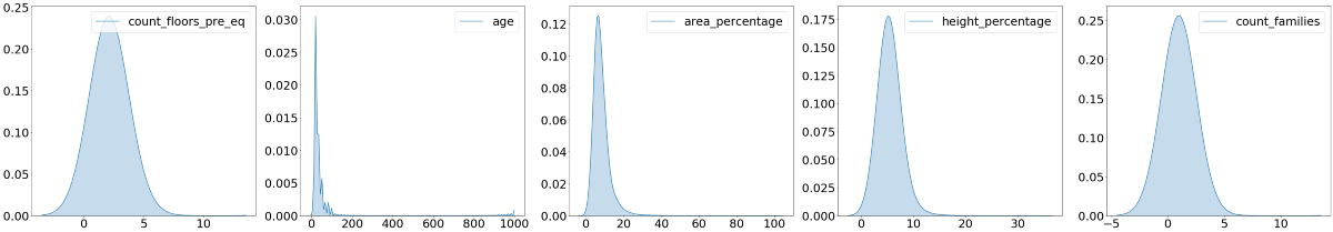
As we can see from the graph above, all the plots exhibit an excessive rightward skew. That means that there are a few observations for each variable which are much higher than the rest of the data. Another way to describe this phenomena would be to say that the mean of the distribution is higher than the median.

As a refresher, skewness describes the symmetry of a distribution. A normal distribution has, as a reference, a skewness of zero, given its perfect symmetry. A high (or low) skewness results from having a few obscurely high (or low) observation in the data, which we sometimes also call outliers. The problem with outliers is manifold, but the most important problem for us is that it hurts the performance of nearly every prediction model, since it interferes with the loss function of the model.

One effective measure to dampen the massive disparity between the observations is to apply the natural logarithm. This is allowed since the logarithmic function represents a strictly monotonic transformation, meaning that the order of the data is not changed when log is applied.

Before being able to apply that measure, we have to deal with the zero values (the natural logarithm of zero is not defined). We do that by simply adding one to every observation before applying the logarithm. Lastly we standardize all variables to further improve our model performance.

# Applying the logs and create new sensible column names
logged_train = dummy_train.loc[:, int_variables]\
    .apply(lambda x: np.log(x+1))
log_names = ["log_{}".format(x) for x in int_variables]
stand_logs = StandardScaler().fit_transform(logged_train)
stand_logs_df = pd.DataFrame(stand_logs, columns=log_names) 
for log_col, int_col in zip(stand_logs_df, int_variables):
    dummy_train.loc[:, log_col] = stand_logs_df.loc[:, log_col]
    dummy_train.drop(columns=int_col, inplace=True)
# Plot the newly created plot log variables
fig, axs = plt.subplots(1, 5, figsize=(60, 10))
for number, ax in enumerate(axs.flat):
    sns.kdeplot(logged_train.iloc[:, number], bw=1.5, ax=ax,
                shade=True, cbar="GnBu_d")
    ax.tick_params(axis="both", which="major", labelsize=30)
    ax.legend(fontsize=30, loc="upper right")
path = (r"{}\logs_int.png".format(output_path))
fig.savefig(path, bbox_inches='tight')

The graph below shows the result of these operations. All distributions look much less skewed and do not exhibit the unwanted obscurely high values which we had before.

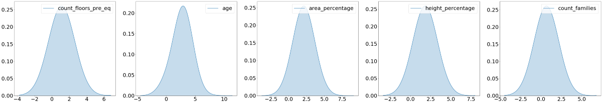
Before moving on, it is important for us to validate that our step taken had a positive effect on the overall performance of the model. We do that by quickly running the new data in our baseline random forest model. Our accuracy is now 73.14, which represents a slight improvement from our baseline model!

Our performance has increased. That tells us that we took a step in the right direction.

05 Geo Variables - Empirical Bayes Mean Encoding

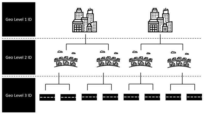
Arguably the most important set of variables within this challenge is the information on where the house is located. This makes sense intuitively: if the house is located closer to the epicenter, than we would also expect a higher damage grade.

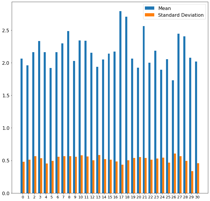
The set of location variables provided within this challenge are threefold. Namely, we get three different geo-identifier with different kind of granularity. For simplicity, we tended to regard the three different identifier as describing a town, district and street (see below).

These geo-identifiers in their initial state are given in a simple numeric format, as can be seen below.

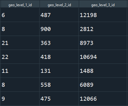
These integer do not prove to by very useful since even though in a numeric format, they do not exhibit any correlation with the target (see graphic below). Meaning that a higher number of the identifier is not associated with higher or lower damage. This fact makes it difficult for the model to learn from this variable.

In order to create a more meaningful variable for the model to learn from these variables, we apply a powerful tool, oftentimes used in data science challenges, called encoding. Encoding is normally used when transforming categorical variables into a numeric format. On first glance we might think that this does not apply to our case, since the geo-identifier is given as a numeric variable. However this understanding of encoders is shortsighted, since whether something represents a categorical variable does not depend on the format, but on the interpretation of the variable. Hence, the variable could gain greatly in importance when undergoing a transformation!

There are a dozen different encoding methods, which are nicely summarized in this blogpost. The most promising method for our case would be something called target encoding. Target encoding replaces the categorical feature with the average target variable of this group.

Unfortunately, it is not that easy. This method may work fine for the first geo-identifier (town), but has some serious drawbacks for the more granular second and third geo-identifier (district and street). The reason is that there are multiple districts and streets which only occur in a very small frequency. In these cases, mean target variable of a group with a small sample size is not representative for the target distribution of the group as a whole and would therefore suffer from high variance as well as high bias. This problem is quite common when dealing with categorical variables with a high cardinality.

One workaround for this problem is a mixture between Empirical Bayes and the shrinkage methodology, motivated by paper [1]. Here, the mean of a subgroup is the weighted average of the mean target variable of the subgroup and the mean of the prior.

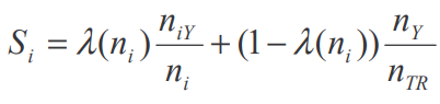
In our example that would mean that the encoded value for a certain street is the weighted average between the mean target variable of the observations of this street and the mean of the district this street is in. (one varaiable level higher). This method shrinks the importance of the potentially few observations for one street and takes the bigger picture into account, thereby reducing the overfitting problem shown before when we had only a couple of observations for a given street.

The question may now arise how we are determining the weighting factor lambda. Using the methodology of the paper in [1], lambda is defined as:

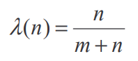
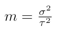
Where m is defined as the ratio of the variance within the group (street) divided by the variance of the main group (district). That formula makes intuitive sense when we consider a street with a few observations which differ massively in their damage grade. The mean damage grade of this street would therefore suffer from high bias and variance (high sigma). If this street is in a low variance district (low tau), it would be sensible to drag the mean of the street into the direction of the district. This is essentially what the m coefficient captures.

It is worth mentioning that the overall model performance in-sample will drop when applying the Empirical Bayes-shrinkage method compared to using a normal target encoder. This is not surprising since we were dealing with an overfitted model before.

Lastly, we run our model again in order to see whether our actions improved the overall model performance. The resulting F1 score of 76.01% tells us that our changes results in an overall improvement.

06 Feature selection

At this point, it is fair to ask ourselves whether we need all the variables we currently use in our prediction model. If possible, we would like to work with as few features as possible (parsimonious property) without losing out too much in our scoring variable.

One benefit of working with tree models is ability to display feature importance. This metrics indicates how important each feature is for our prediction making. The following code and graph displays the variables nicely.

fimportance = main_rmc_model["model"].feature_importances_
fimportance_df = pd.DataFrame()
fimportance_df.loc[:, "f_imp"] = fimportance
fimportance_df.loc[:, "col"] = dummy_train.columns
fimportance_df.sort_values(by="f_imp", ascending=False, inplace=True)
fig, ax = plt.subplots(1, 1, figsize=(12, 24))
ax = sns.barplot(x="f_imp", y="col",
                data=fimportance_df,
                palette="GnBu_d")
ax.tick_params(axis="both", which="major", labelsize=20)
ax.set_xlabel("Feature Importance in %", fontsize=24)
ax.set_ylabel("Features", fontsize=24)
path = (r"{}\feature_importance.png".format(output_path))
fig.savefig(path, bbox_inches='tight')

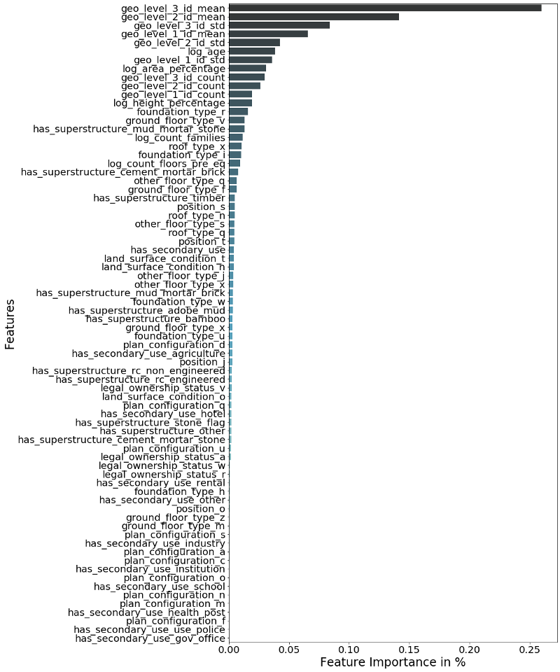
As we can see from the graph above, the most important variables to predict the damage grade of a house is the average damage grade of the different geo-locations. This makes sense, since the level of destruction of one house is likely to be correlated with the average damage of the houses around.

06.1 Low importance of binary variables

The feature importance also shows that nearly all binary variables have a low feature importance, meaning they are providing the model with little to no predictive information. In order to understand that better we take a look into the average of all binary variables, which is a number between zero and one.

binary_variables = variable_dict["binary_variables"]
mean_binary = pd.DataFrame(dummy_train.loc[:, binary_variables].mean())
mean_binary.loc[:, "type"] = mean_binary.index
fig, ax = plt.subplots(1, 1, figsize=(12, 12))
ax = sns.barplot(x="type", y=0,
                data=mean_binary,
                palette="GnBu_d")
ax.tick_params(axis="both", which="major", labelsize=16)
ax.set_xticklabels(mean_binary.loc[:, "type"], rotation=90)
path = (r"{}\binaries_mean.png".format(output_path))
fig.savefig(path, bbox_inches='tight')

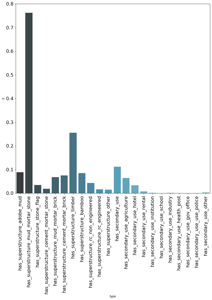
As can be seen above, nearly all variables have a mean below ten percent. That implies that most rows are equal to zero, a phenomenon we normally describe as sparsity. Furthermore, it is visible that the binary variables with an average above ten percent have also a higher feature importance within our prediction model.

This finding is in line with the fact that tree models, and especially bagging models like the currently used Random Forest, do not work well with sparse data. Furthermore, it can be said that a binary variable which is nearly always zero (e.g. has_secondary_usage_school), simply does not carry that much meaning given the low correlation with the target.

Using cross-validation, we find that keeping features which have an importance of minimum 0.01%, leaves us with the same F1 score compared to using all features. This leaves us with 53 variables in total. This number, relative to the amount of rows we have (260k) seems reasonable and therefore appropriate for the task.

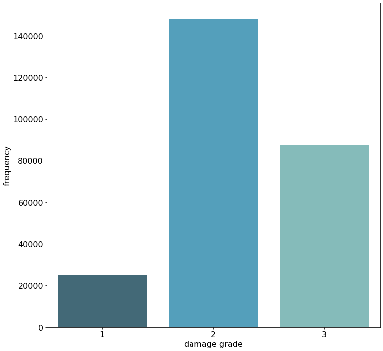
07 Imbalance of damage grades

One of our key learnings in this challenge was how to handle the massive imbalance of the target variable. Namely, not to touch it at all!

When looking at the chart below, we can see that the first damage grade does not nearly appear as often as the second damage grade. It may be tempting now to apply some over- or undersampling to the data in order to better balance the data and to show the model an equal amount of each damage grade. The main problem with this approach is that the test data comes from the same (imbalanced) distribution as the training data, meaning that improving the accuracy score for the lowest damage grade, through sampling methods, comes with the costs of a lower accuracy of the highest occurring, and therefore more important damage grade two.

07.1 Performance & Concluding Remarks

Following all steps of this blogpost (with a few minor tweaks and hyperparameter tuning) led us to place 34 out of 2861 competitors.

We are overall quite happy with the placement, given the amount of work we put in. This challenge touched on many different aspects and taught us a lot. Data Science Challenges are a perfect learning opportunity since they are very close to real life problems.

We are looking forward to our next one!

References

[1] Micci-Barreca, Daniele. (2001). A Preprocessing Scheme for High-Cardinality Categorical Attributes in Classification and Prediction Problems.. SIGKDD Explorations. 3. 27–32. 10.1145/507533.507538.