Feature Creation for Real Estate Prices
Feature Creation for Real Estate Price Prediction This post elaborates on feature engineering for Spanish real estate price prediction.
This post is structured as follows.
- Importance of feature engineering
- Proximity of larger cities
- Hyped cities
- Temperature Data
- Conclusion
01 Importance of feature engineering
Within Machine Learning, the big hype is normally centered around fancy prediction models and opportunities for incremental improvements through hyperparameter tuning. Equally important, if not even more important, are the features which are fed into the model. Feature creation and selection are the true heroes of Machine Learning- and often times responsible for much higher gains in performance than hyperparameter tuning. Finding relevant and well-defined input variables can boost the accuracy of any model significantly.
Creativity and data availability are the “only “ limits when it comes to feature creation. Deciding which features to implement depends on the particular prediction task. Our task is to build a prediction model for real estate prices. The question is then: “what factors influence are most likely to influence the price of real estate, and how can we help our model to better understand these?” We ended up with three implementable ideas.
The first one is the proximity of a property to a larger city. Living closer to a denser populated city comes with the perks of being able to take advantage of everything a city has to offer and should therefore also impact the price of an property.
The second variable is an indication of whether the property’s location is one of the hotspots within Spain. This feature tries to capture the superior attractiveness and lifestyle of these cities.
The last variable is the climate in the property’s area. Spain is espcially attractive as a retirement destination because of its Mediterranean climate and endless sunshine. The variation of climate within the country is also likely to explain some variation within price.
This post elaborates on all these variables and shows how they were implemented. For each variable, we start by motivating the theoretical significance of the variable. We then show the methodology and implementation of the code.
02 Proximity to larger cities
02.1 Motivation
The idea for this variable came when thinking about small apartments in large cities like London or New York. The price tag of small apartments in New York is mind boggling compared to what you get. You end up paying multiple thousands per month for a small bedroom and an even smaller bathroom. The amount of money paid in rent (or purchase) of such an apartment can buy significantly more property somewhere else.
The reason why these prices are justifiable in New York or London is the location in the midst of a major global city. This characteristic of a property, namely being in a reasonable range of such a city (and how many such cities are close by) is what we try to capture for our Spanish real estate data.
02.2 Methodology
Two different kinds of feature variables are created. The first one is a count of how many cities are in a certain radius of a property. The second one is how close the nearest city with more than 100,000 habitats is. The latter should give an indication how rural the estate is and corrects for a potentially incorrectly chosen radius when constructing the first variable.
Furthermore, we distinguish between the kind of city. Living close to New York may be better (or worse) than living close to a 50,000-inhabitant city. Regardless of the effect on price of these different cities, meaning regardless of whether one has a stronger or weaker effect, we assume that the effect is different in magnitude. In order to allow for a different effect on price, we distinguish between different city sizes. Our definitions are in line with the commonly applied settlement hierarchy. Hence we define:

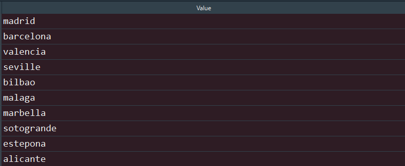
This variable creation requires knowing the city names, as well as the location of every city with more than 100,000 inhabitants. This information is taken from here. The data looks like this:

According to our source, we find two cities with more than one million inhabitants, ten cities between 300k and 1m habitats and 76 cities with a population between 100k and 300k. In order to keep the type of city groups to a minimum (medium, large and metropolis) we assigned Madrid to the metropolis definition as well (even though it has 200k more habitats than the formal definition of a Metropolis city).
The next step now is to count how many of these cities shown above are within a certain radius of each property. To do that we need two things: a radius definition, and a function to calculate the distance between the two locations.
We use a radius of 30 kilometers euclidean distance (the way the crow flies). This number seems sensible given that distance on the road would then be probably around 50 kilometers, which represents approximately a one-hour drive with a car. As this radius was chosen arbitratily, we tested several different radius lengths in order to conduct sensitivity checks. We found only a negligible variation in the results with these checks.
The code for calculating distances between two locations given their longitude and latitude information is the following:
def dist_bool(list1, list2, radius):
# Separation of the longitude and latitude data
    lat1, lon1 = list1[0], list1[1]
    lat2, lon2 = list2[0], list2[1]
# Earth radius in km
    R = 6371
#conversion to radians
    d_lat = np.radians(float(lat2)-float(lat1))
    d_lon = np.radians(float(lon2)-float(lon1))
    r_lat1 = np.radians(float(lat1))
    r_lat2 = np.radians(float(lat2))
#haversine formula
    a = np.sin(d_lat/2.) **2 + \
        np.cos(r_lat1) * np.cos(r_lat2) * np.sin(d_lon/2.)**2
# Calculate distance between two points
    haversine = 2 * R * np.arcsin(np.sqrt(a))
# Checking whether it is still within the radius
    within = radius >= haversine
# Returning the results
    return within
02.3 Results
The summary statistics of these two features are visible below. We see that 8% of all properties are within a 30 kilometer range of a metropolis. That is sensible given the high amount of smaller cities that are essentially suburbs of either Madrid or Barcelona. We find furthermore that the average amount of medium cities within a 30 kilometres radius for all properties is around two on average.
One should be cautious with the interpretation of that result, given that one observation had around 26 medium sized cities within its radius. This is likely to be the case of cities which are located within the Madrid Provence, where all smaller suburbs around Madrid are counted as an independent city. This fact can alter the statistic.

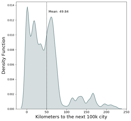
The second variable is the measure of how many kilometres away (euclidean distance) from the property is the closest city with more than 100k habitats.
The summary statistics as well as the distribution plot below show us that a considerable amount of estates within our data are well connected, with more than half of our observations being less than 50 kilometers away from a larger city.

03 Hyped cities
03.1 Motivation
Real Estate is an interesting mixture of art and science. Nobody can truly explain why one area of the city is so much more popular than another by just looking at a map. Often times certain districts or even entire cities are hyped. This subjectivity in attractiveness is difficult to encapsulate in a measurement. One approximation would be to see what well known magazines report as hyped cities is districts, as we’ve done here.
03.2 Methodology
In order to understand what cities are currently the best places to live, we use this website which ranks as one of the best expatriate publications online. We again use webscraping to obtain all the locations which, according to the website, are the best places to live. The code below shows how exactly this is done.
# The link where to find all the real estate
url = "https://expatra.com/guides/spain/best-places-to-live-in-spain/"
# Requesting the sites content
page = requests.get(url)
soup = BeautifulSoup(page.content, "html.parser")
# Getting the table with all places in spain
table_html = soup.find_all('li', class_='ez-toc-page-1')
# Getting all the cities
cities = [x.text for x in table_html]
cities = cities[1:-1]
# Changing all city names to lower case
cities = [x.lower() for x in cities]
03.3 Results
After scraping we have a list of cities. As the last step we then create a dummy variable which indicates whether a property is located in any of these hyped cities.
04 Temperature data
04.1 Motivation
One of the main reason to obtain a Spanish property for many foreigners is probably the weather. Spain, given its location, is one of the warmest places within Europe. It is therefore likely to be of high interest for a buyer how often it rains, what the average temperature is and potentially how windy it is.
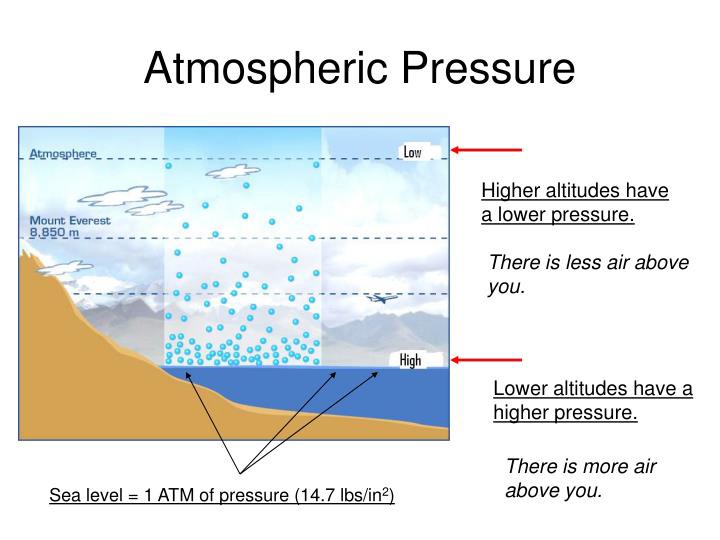
Furthermore, given that the air pressure is higher for areas closer to sea level (explanation below), this variable may kill two birds with one stone, serving also as a proxy for distance to the sea. Including this variable also assumes that a buyer is more likely to pay a premium to live closer to the sea.

04.2 Methodology
Since it was not possible to find good average climate data for each city in Spain, we had to change strategy. Instead, we found climate data for different weather stations in Spain, namely information of 114 weather stations scattered around the country. Using their longitude and latitude information we plotted the different weather stations below in a scatter plot. The graph shows nicely that we have weather stations all around Spain, even with several on in Gran Canaria.

The task is now to calculate the average climate information and then find the weather stations closest to every property. This is done by using the distance calculator shown earlier in this post.
The question arises how many years should be used to average the climate data. The accepted convention to calculate the average climate is 30 years, according to scientific sources. Our data starts as early as 2012. We then use 30 years of observations from 2012 backwards. Below we can see the results of these calculations for some example weather stations.

05 Conclusion
Feature creation is one of the most important steps when building prediction models. Feature engineering also often proves much more important for model performance than hyperparameter tuning.
However, feature engineering also has plenty of drawbacks. From our perspective, there are three main challenges that arise during the process of feature creation.
It begins with having an idea what kind of feature could be potentially useful. Next and even more critical is the availability of data. In our example we could not find climate data for every city in Spain and therefore had to use weather stations instead. This alternative source is nevertheless better than not including any weather data and represents a good compromise.
The last difficulty is data handling. Oftentimes scraped data or csv imports come in inconvenient formats and always have to be cleaned and prepared before being useful in modeling.
The potential unrewarding moment comes when the model shows insignificant importance of the feature you engineered. Unfortunately, this problem is not possible to mitigate beforehand - it’s hard to predict how important a feature will be for a model.
In the next post, we feed the features created here and the original features from the real estate advertisements into several prediction models to assess the importance of all features in predicting price.

