NLP with Real Estate Advertisements - Part 2
Applying our NLP feature vector to the Gradient Boosting model.
Recall from Part 1 of analyzing real estate advertisement descriptions that we prepared our data for modeling by splitting it into tokens and removing common real estate stop words. These initial steps made it easier to visualize our text data, but before we can use the text data in models, we need to put our words in some kind of numeric format. This is because ML models can only take numeric data as inputs.
In this article, we show how we prepared the data for use in machine learning models using a TF-IDF vectorizer, and how these features impact the model.
This article proceeds as follows:
- TF-IDF vectorization of text features
- Inclusion of TF-IDF features in XG-Boost model
- PCA for dimensionality reduction of text features
- Conclusion
01 TF-IDF Vectorization of Text Features
TF-IDF stands for Text Frequency-Inverse Document Frequency. It is a ratio of how often a word appears in a given text, compared to how often that word appears in all texts.

To understand how TF-IDF vectorization works, we’ll look at a simplified example. In our example, we have 2 short real estate advertisement descriptions where stopwords have been removed.

Note that Advertisement 1 contains 6 words, whereas Advertisement 2 only contains 5 words. Both advertisements contain the term “for sale”, though these words are in a different position in each of the advertisements.
To calculate the TF-IDF score for each advertisement, we first need to calculate the inverse document frequency, IDF, for each word. The first step in calculating IDF is to divide the total number of documents, N, by the number of documents containing the given word. Then, this inverse fraction is logarithmically scaled.

Note that only the words “for” and “sale” have a lower IDF score, since they are the only words that appear in both documents. All other words only appear in one document each, so they each receive the same score.

Next, for each document, the term frequency (Tf)is calculated. This is simply a count of how often each term appears in the document. Since each advertisement only has 5 or 6 words and each word only appears once, the term frequency is never higher than 1 for each document.
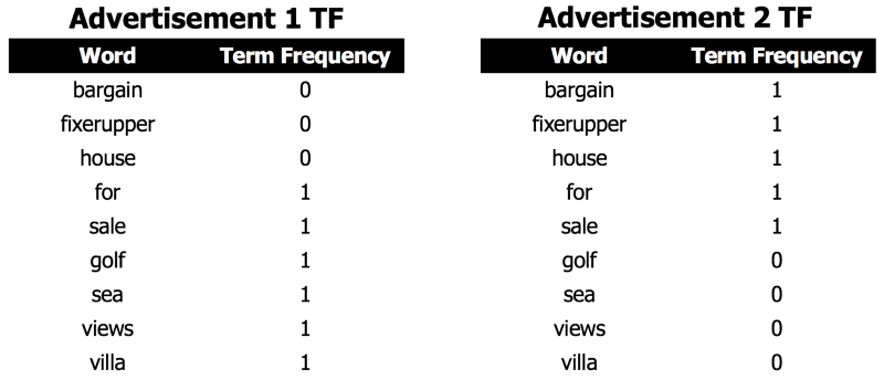
With term frequency for each document, a matrix multiplication is done with the term frequencies and inverse document frequencies to arrive at the final TF-IDF vector for each document.
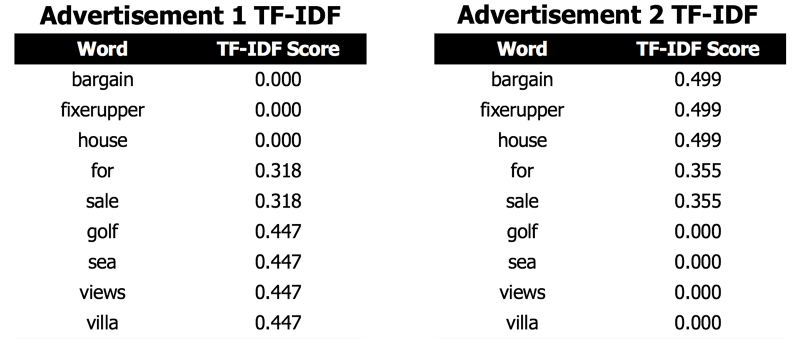
TF-IDF scores for each advertisementNote that the scores for the words that appear in Advertisement 2 receive a are always a bit higher than the scores for the words in Advertisement 1. Since Advertisement 2 contains fewer words than Advertisement 1, each word is counted as relatively more important.
To better understand how TF-IDF vectorizes our Spanish real estate data set, we’ll look at the same example we used in Part 1 of analyzing subsets of “cheap” and “expensive” homes in our data. Recall from Part 1 that we defined “cheap” homes as the most inexpensive 5% of our data, those under €75,000, and the “expensive” homes as the most expensive 5% of our data, those above €1.7 million.
The TF-IDF scores for the cheapest and most expensive properties are shown below. The TF-IDF scores shown are the sum of all scores for the word for each advertisement that was included in the “cheap” or “expensive” category.
cheap_property_TF_IDF_scores =
[('town', 122.68691198513302),
('village', 85.8624409730794),
('like', 84.06423081796622),
('need', 72.47179535414357),
('terrace', 71.42720081950334),
('large', 68.99777093615201),
('townhouse', 68.9844994563653),
('family', 63.417517090288484),
('space', 62.07432797305012),
('build', 60.04214108962623),
('distribute', 58.4163261755536),
('street', 58.24476489238489),
('situate', 57.41386787457465),
('close', 54.99513021566562),
('child', 53.1243500223459),
('good', 50.895927008310515),
('ideal', 50.66644469452883),
('size', 47.013810045109445)]

expensive_propertytfidf_list =
[('villa', 217.80253394946453),
('view', 147.775603675447),
('sea', 124.69304169060362),
('build', 105.68834130627678),
('luxury', 98.60403119678404),
('exclusive', 93.06584872644288),
('modern', 85.62951731804527),
('beautiful', 85.62351304555642),
('design', 74.60755941148277),
('offer', 70.22014987779879),
('minute', 67.10389304885832),
('beach', 64.12585728939085),
('unique', 63.49425807437234),
('spectacular', 61.895439206382186),
('high', 58.92975340566454),
('town', 58.88803267728475),
('large', 57.488549315155126),
('stunning', 55.85328236142857),
('quality', 53.57454240044263),
('style', 51.88205837353272)]
These words are many of the same words that were included in the “cheap” and “expensive” wordclouds.
The TF-IDF vectorizer has a few hyperparameters that, when adjusted, change the vector they create. Perhaps the most important of these hyperparameters are min_df and max_df. Min_df defines the minimum number of documents in which a word must appear in order for it to be counted. Setting this value to 0.05, for example, means that words which appear in only 5% of the documents, or less, are not included. In the context of real estate listings, this would likely exclude words like a particular street name or seldom-used adjective that only occur in one advertisement and can prevent overfitting. Max_df, on the other hand, defines the maximum number of documents in which a word can appear. This prevents words which appear in almost every listing from being included in the feature vector. Terms like “for sale” would likely be excluded with this metric.
Below is a list of some of the words which were excluded with the min_df=0.02 and max_df=.90 with our real estate dataset. This means we excluded words that don’t exist in at least 2% of all property advertisements, as well as words that exist in more than 90% of all advertisements.
selected_exluded_words = ['kennel', 'ciencias', 'mayores', 'castiilo', 'montroy', 'worthy', 'furniture', 'ricardo', 'fend', 'españa', 'iron', 'rotas', 'sans', 'alike', 'portals', 'dividable', 'majestically', 'ladder', 'communicate',  'orientation',  'grass',
'visited', 'identify', 'setting', 'café', 'specimen', 'dorm', 'unsurpassed', 'later', 'tarred', 'oil']
Limiting the NLP features considered in this way decreased the dimensionality of our TF-IDF feature matrix from 13,233 columns to 158 columns, meaning 158 terms were then used to train the model. This drastically decreases the dimensionality of the NLP feature vector, as well as decreasing potential noise.
02 Inclusion of the NLP features in the XG-Boost model
These 158 additional features were then fed in as additional training features to the XG-Boost model. The model’s hyperparameters were also tuned using GridSearchCV.
The improvements in performance were quite surprising. The best MAPE score achieved on the first, and hardest to predict, quintile of data using the baseline features was a 46.74 % error. Including the 158-feature TF-IDF matrix, this error was cut nearly in half to 27.01%.
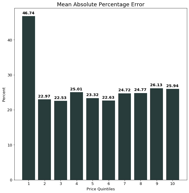
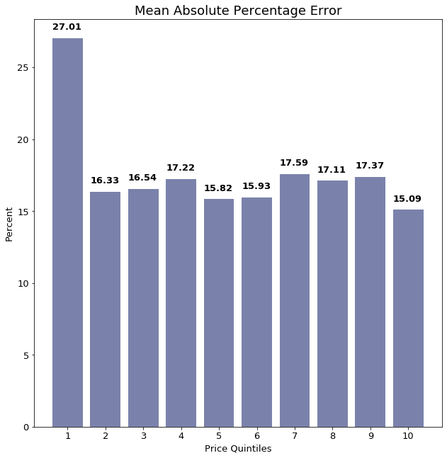
We further investigated the impact of the additional NLP features by looking at observations where the NLP features led to especially large model perfomance gains.
We identified almost 50 properties where the prediction improvement using NLP was more than 100%. Of these, nearly all were properties where the “logs-only” model had predicted much too high.
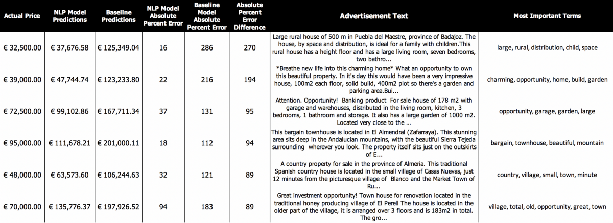
The word “opportunity” seems to be one that really helps the model learn that a property should be valued lower. The inclusion of the words “town”, “village” and “rural” also fits with our understanding of words associated with inexpensive properties found in Part 1.
The inclusion of NLP features improved the overall model performance drastically. However, there were some individual observations where including the NLP features increased the absolute percentage error for those properties. Upon closer investigation, many of these contained no description. This then makes sense that the model trained on a feature set which includes NLP features did a worse job predicting these observations with no description. The model now relies more on the NLP features and less on the original features. So when there are no NLP features, the model does a worse job of predicting since it is putting less weight on the original features.
03 Dimensionality reduction of text features using PCA
It’s clear that the inclusion of NLP features greatly improved model performance. However, the number of features it adds is quite large - the NLP feature vector adds 158 additional features.
One of the most common methods for reducing dimensionality in input features is Principal Component Analysis, or PCA. PCA works by projecting the features onto a smaller (lower-dimension) vector space.
We started with mapping the 158-NLP feature matrix onto an 8-feature PCA feature space.
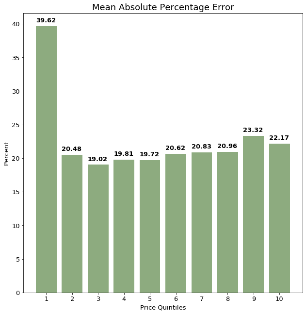
The MAPE in each price quintile is lower (better) than using the logged features alone, but significantly higher than when using all 158 NLP features.
Conclusion
Adding the full 158 NLP features greatly improved model performance. Using only 8 PCA principal components still improves model performance over the original model, but not nearly as much as including all 158 features.
The decision to include all 158 features or only the 8 PCA features depends on what is needed from the model. In this case, it is likely that the gains in performance outweigh the slightly longer prediction time caused by including all NLP features.
In the next article, we summarize the work done so far and look forward to potential next steps.

