Signal Processing - Engine Sound Detection
Detecting the engine-brand from a Formula 1 car by its sound using Neural Networks
Formula 1 is not everybody’s cup of tea. Whereas some celebrate risky takeover maneuvers, others only see dangerous driving in spaceship-looking vehicles. One particularly divisive aspect of the sport is the incredibly loud and distinct noise made by the cars. Even though the FIA banned the infamously loud V12 in the year 2000, Formula 1 cars are not known to go by unnoticed.
For many opponents of the sport all engines sound the same. But do they really? This project tries to predict the engine-brand using sound data.
Overview
This blogpost elaborates on how to build a sound-recognition model from scratch using a Neural Network. Given that we need to process audio data before the Neural Network can be trained on it, several sound concepts and terminology are introduced to give the reader a better understanding.
The post starts by elaborating on where from and how the data was collected. Afterwards, we cover some audio-related terminology before diving into the practical implementation of signal processing in Python.
After the bulk-processing of the audio data is conducted, we focus our attention onto the implementation of the neural network using tensorflow. As the last step we then implement our prediction onto some test-data and create a montage video, which is also used as the title image of this blogpost.
Data Collection
In order to build a model that predicts which sound belongs to which engine, we need labelled sound-data. Labelling means we know which engine-brand produced which sound.
Obtaining Formula 1 content proved to be relatively easy through their official Youtube Channel. Here we find a compilation of videos labelled Pole Laps. Before each race in Formula 1, as in every other motorsport, every driver undergoes a procedure called Qualifying where each driver tries to complete the track in the shortest possible time. The person who wins this competition gets rewarded with the Pole Position. This term, which originates from horse racing, describes the most favorable position a driver can think off for the actual race - namely starting from the very front.
Given that the lap which sets the quickest time, the so called Pole Lap, is interesting to watch for many, the official Formula 1 channel uploaded an on-board video taken from the care from this lap for every race. Below we find a compilation of short snippets from these videos.
We use these qualifying lap videos as they contain only one car, making the sounds data pure. In the actual race where many cars are driving, it would be much more difficult to identify and separate out the individual sounds of each engine.
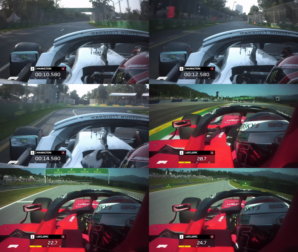
Next to be very entertaining to watch, these videos are particularly useful for our task. That is because the data is labelled (we know which engine-brand is driving in which video) and the data is relatively free from any noise.
Furthermore, in the racing year 2019 two engine-brands were taking turns in winning the Qualifying - Ferrari and Mercedes. To be exact, out of 21 Qualifying, Mercedes and Ferrari won 10 and 9 of these, respectively.
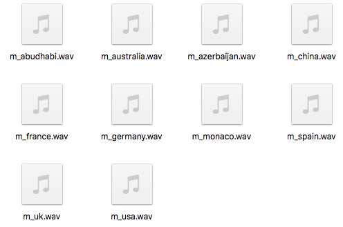
Since we are solely interested in the sound of these videos we extract the sound information from these 19 videos and save them in a wav-format.
Sound Data - First Steps
The processing of sound data might be a bit unfamiliar for some, therefore the following section explains the fundamentals of sound data.
We’ll start by answering the first fundamental question - what is sound? Sound could be described as simply the vibration of an object. The vibrations then cause the oscillation of air molecules. We can hear this sound as soon as these vibrations hit our ear.
Sound is a continuous variable, meaning that we have an infinite amount of information, or data points, per second. This actually represents a bit of a problem when trying to store that information - we have to turn this continuous signal into a discrete one. That process is called Analog to digital conversion (ADC).
ADC does two things: first, it samples the sound information, and second, it quantifies the information at each sampling point. The sampling frequency is measured in hertz and describes how often we would like to store sound information per second. The more samples we take within a second, the smaller the overall loss of information. That does not mean though that a higher sampling rate is always better though. A classical CD has around 22,050 hertz. The reason for this seemingly arbitrary number is the hearing range for humans, which is around 20,000 hertz. Hence, for humans the sampling rate of a CD is more than sufficient to appreciate the sound.
After knowing how often we would like to sample per second we should talk about what exactly we store. Here the term quantization comes into play. Quantization assigns a value to each sound signal we extract. Given that sound information has a continuous value and we have to store that information in a discrete way for a computer to store it. For example, if the signal has a value of 2.234253243… (meaning a never ending number), we will round to e.g. 2.23. This, of course, leads to some sort of a rounding error. How high this error is depends on the resolution of the sound. This resolution is measured in bits (also referred to as bit depth). A CD has a bit depth of 16, which is sufficiently high for the human ear.
Wave-plots and related Terminology
After covering how sound-information is stored, it is now time to talk about how the actual processing of sound-information works. We start by introducing the probably most common sound-visualization - the wave-plot.
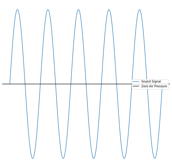
A wave-plot displays the sound-signal as a function of time. Technically put, a wave-plot shows the deviation of the zero-line in air pressure. A wave-form, even though looking relatively simple, carries a lot of further relevant information like frequency, amplitude, intensity and timbre of the sound. These attributes shape how exactly the wave-plot looks.
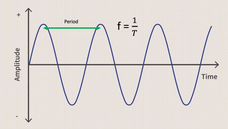
These additional attributes in the wave-plot are extremely important for understanding sound, so we’ll look at them more closely and explain their meaning. Frequency is the inverse of the amount of time that elapses between two peaks of a soundwave, called periods. The graph below illustrates that concept, where f denotes the frequency and T the time of a period. Overall, a higher frequency leads to a higher-pitched sound, whereas a lower frequency leads to a lower/ deeper sound. Unlike the graphic below, most sounds in real-life are not that nice and easy. Most of the time we face a so called aperiodic sound, which consists out of many different frequencies laying on top of each other.
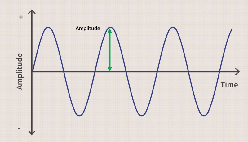
Amplitude, on the other hand, quantifies the perturbation of the air pressure. A higher perturbation signifies more energy being transmitted through the soundwave. This results in a louder sound. A low amplitude results then, consequently, in a more quite sound.
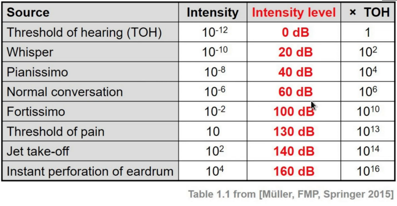
Intensity is formally measured in sound power per unit area. Given the incredibly large range of sounds that a human ear is able to hear, this variable uses a logarithmic scale. Furthermore, it is important to know that this variable is measured in decibels. Below we find a table which gives us some sort of indication about the magnitude of decibels. Our Formula 1 car has an intensity of 140 decibels and is therefore relatively close to the threshold of permanent hearing damage.
The last concept of importance is called timbre. This variable is probably the most abstract concept we encountered so far. It is normally described as the color of the sound. It describes the difference in sound holding frequency, intensity and duration constant. The importance of the variable becomes clear when trying to distinguish a trumpet and a violin which play the exact same sound. It is exactly this variable which will play a crucial role within our task of identifying the engine-brand.
After covering the most important concepts of sound, it is now time to take a look at our data by building wave-plots. We start by building one sound-wave for each engine-brand, meaning one for Ferrari and one for Mercedes.
We start by importing all the relevant packages and defining the paths on our computer. Furthermore, we build a dictionary which specifies the location of the two audio files and the color we would like to draw them in.
# Packages
import librosa, librosa.display
import numpy as np
import matplotlib.pyplot as plt
import os
# Paths
main_path = r"/Users/paulmora/Documents/projects/formula"
raw_path = r"{}/00 Raw".format(main_path)
code_path = r"{}/01 Code".format(main_path)
data_path = r"{}/02 Data".format(main_path)
output_path = r"{}/03 Output".format(main_path)

# Specifying plotting information
dict_examples = {
    "ferrari": {
        "file": r"{}/ferrari/{}".format(raw_path, "f_austria.wav"),
        "color": "red"
    },
    "mercedes": {
        "file": r"{}/mercedes/{}".format(raw_path, "m_australia.wav"),
        "color": "silver"
    }
}
When importing the sound file we have to specify the sample rate. As discussed in the beginning of the blog-post, a Sample Rate of 22,050 hertz is more than sufficient.
The go-to sound processing package in Python is called librosa. This package has a handy command for calculating and plotting the wave-plot.
fig, axs = plt.subplots(nrows=1, ncols=2, sharey=True, figsize=(20, 10))
SR = 22_050
axs = axs.ravel()
for num, team in enumerate(dict_examples):
    signal, sr = librosa.load(dict_examples[team]["file"], sr=SR)
    dict_examples[team]["signal"] = signal
    librosa.display.waveplot(signal, sr=sr, ax=axs[num],
                             color=dict_examples[team]["color"])
    axs[num].set_title(team, {"fontsize":18})
    axs[num].tick_params(axis="both", labelsize=16)
    axs[num].set_ylabel("Amplitude", fontsize=18)
    axs[num].set_xlabel("Time", fontsize=18)
fig.savefig("{}/waveplot.png".format(output_path),
            bbox_inches="tight")
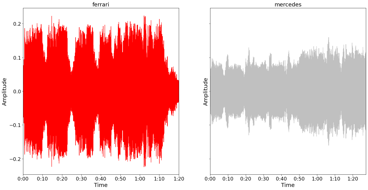
Listening to one of the videos, one quickly notices that the engine is as its loudest when driven full-speed. This, probably not very noble finding, explains the aperiodic behavior of the wave-plots above. It is likely that every systematical temporary drop in amplitude is due to a time when the car slowed down a.k.a when facing a corner.
Looking at the two plots above it looks like the Ferrari engine is significantly louder than the Mercedes engine. It would be important to check whether that is a systematic finding, or whether a specific one. For that reason we plotted the wave-plots for all races.
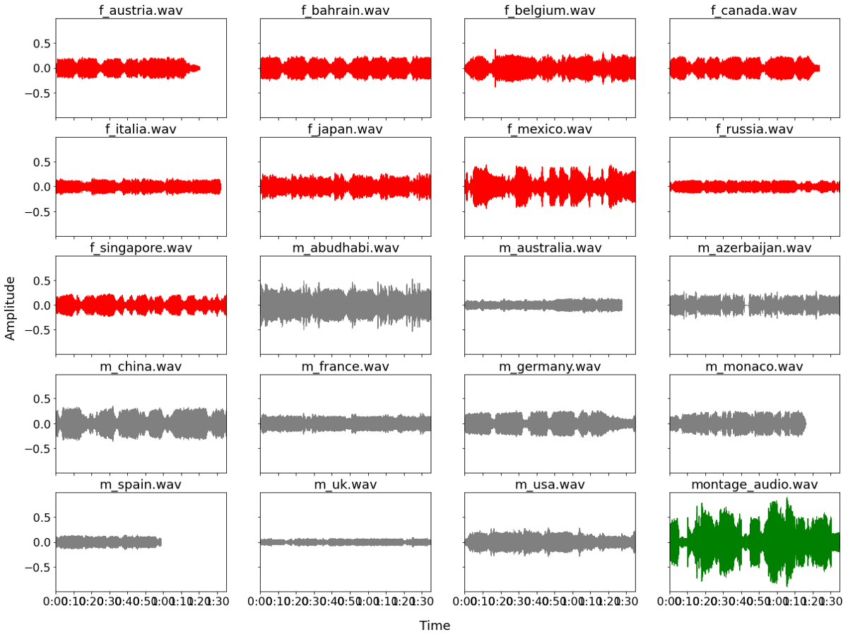
The plot above shows us that identifying which engine-brand a sound belongs is not as easy as just looking for the higher amplitude/ louder sound. The plot tells us that whether a sound is relatively loud or quite is somewhat random and not specific to an individual engine.
The pondering question now is what we can learn from the wave-plots we saw before. Even though a wave-plot captures a lot of information, most of it is not entirely visible to us at that point. As the next step we will take a deeper look into the different frequencies of our sound. This is done by using a so-called Fourier Transform.
Fourier Transform
A Fourier Transform describes the method of decomposing complex sounds into a sum of sine waves, oscillating at different frequencies. To understand what that means, it is important to acknowledge that every complex sound (e.g. not a simple sine wave) consists out of a sum of many smaller sounds.
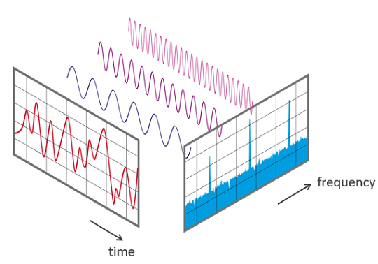
The Fourier Transform is particularly interested in the amplitude of each frequency. That is because the amplitude tells us the magnitude by how much a specific frequency contributes to the overall complex sound.
A good comparison to understand that context better would be the creation of a cooking sauce. A sauce has a certain taste which is driven by its different ingredients. In the beginning it might seem very difficult to tell which and by how much each spice is contributing to the overall taste. A Fourier Transform tells us exactly that. It splits up the sauce into the different components and tells us how much of which spice was used to create the overall sauce and taste.
Coming back to our Formula 1 car-sound example. When applying a Fourier Transform on our sound information from before, we end up with the following two, so called, power-spectrum. The code below shows how to create the power-spectrums for our problem:
fig, axs = plt.subplots(nrows=1, ncols=2, sharey=True, figsize=(20, 10))
axs = axs.ravel()
for num, team in enumerate(dict_examples):
    # Calculating the fourier transform
    signal = dict_examples[team]["signal"]
    fft = np.fft.fft(signal)
    magnitude = np.abs(fft)
    frequency = np.linspace(0, sr, len(magnitude))
    left_frequency = frequency[:int(len(frequency)/2)]
    left_magnitude = magnitude[:int(len(frequency)/2)]
# Plotting results
    axs[num].plot(left_frequency, left_magnitude)
    axs[num].set_title(team, {"fontsize":18})
    axs[num].tick_params(axis="both", labelsize=16)
    axs[num].set_ylabel("Magnitude", fontsize=18)
    axs[num].set_xlabel("Frequency", fontsize=18)
    axs[num].plot(left_frequency, left_magnitude,
                  color=dict_examples[team]["color"])
fig.savefig("{}/powerspectrum.png".format(output_path),
            bbox_inches="tight")
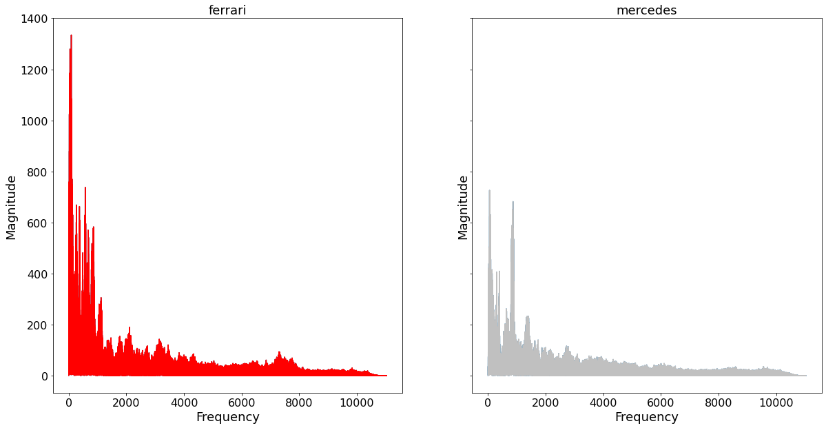
The plots above show us the Magnitude as a function of Frequency. We can see that the main sound for a F1 car is to be found in the lower levels of frequency.
A power-spectrum has one central weakness. Namely, the loss of the time domain. A power-spectrum shows us which frequency drives the overall sound, for the entire soundtrack. That static behavior, of course, a problem since music is a time series and changes over time are crucial.
The solution to that problem is something called a Short Time Fourier Transform which is explained in the next section.
Short Time Fourier Transform
In order to fight the static behavior of the power-spectrum, a dynamic version is created, namely a Short Time Fourier Transform (STFT). A STFT computes several Fourier Transforms at different intervals. This has the benefit that the time information is persevered without losing any of the benefits of a regular Fourier Transform.
To apply a Short Fourier Transform in Python we need to specify several variables, namely the n_fft and the hop_length. The n_fft denotes the number of samples for number of samples we use to calculate each Fourier Transform. It can be regarded as the size of the moving window over time. The hop_length, on the other hand, denotes how much we shift to the right after conducting one Fourier Transform. The common values for these variables are 2048 and 512 samples, respectively.
A STFT results in something called a spectogram, which is an important concept within the realm of signal processing, as it compromises information about time (x-axis), frequency (y-axis) and magnitude of sound (color). The following code shows how to implement such a STFT for our example.
n_fft = 2048  # Window for single fourier transform
hop_length = 512  # Amount for shifting to the right
fig, axs = plt.subplots(nrows=1, ncols=2, sharey=True,
                        figsize=(20, 10))
axs = axs.ravel()
for num, team in enumerate(dict_examples):
    signal = dict_examples[team]["signal"]
    stft = librosa.core.stft(signal, hop_length=hop_length,
                             n_fft=n_fft)
    spectogram = np.abs(stft)
    log_spectogram = librosa.amplitude_to_db(spectogram)
    plot = librosa.display.specshow(log_spectogram, sr=sr,
                                    hop_length=hop_length,
                                    ax=axs[num])
    axs[num].tick_params(axis="both", labelsize=16)
    axs[num].set_title(team, {"fontsize":18})
    axs[num].set_ylabel("Frequency", fontsize=18)
    axs[num].set_xlabel("Time", fontsize=18)
cb = fig.colorbar(plot)
cb.ax.tick_params(labelsize=16)
fig.savefig(r"{}/short_fourier.png".format(output_path),
            bbox_inches="tight")
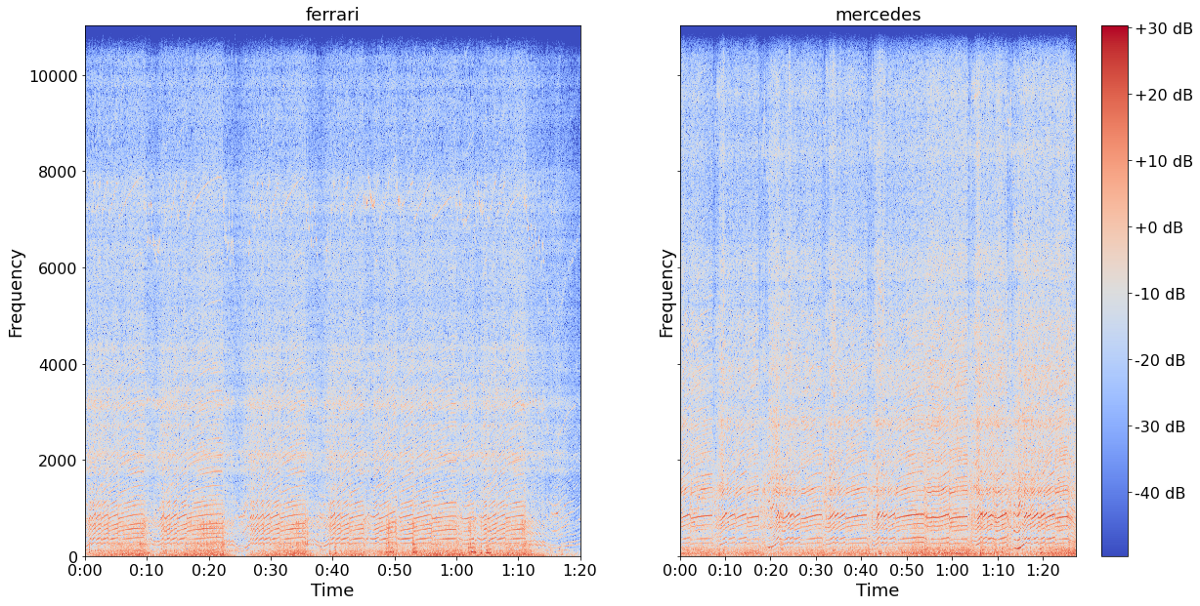
Looking at the chart above, the benefit of the spectogram over the power-spectrum becomes apparent. Whereas in the power-spectrum we were only able to tell that the sound-piece contains strong low-frequency sounds, the spectogram can also tell us now when in time the frequencies occur.
For example it becomes apparent that the Mercedes Engine exhibits overall somewhat more intense higher frequencies compared to the Ferrari engine. That could be potentially helpful for the model to depict the differences.
The information we gathered so far provided us with a lot of insights. However, so far we do not have anything to feed into a prediction model. The next step will take care of that problem. For that we introduce the concept of MFCCs.
MFCCs
Arguably even more important than the spectogram is the concept of the Mel Frequency Cepstral Coefficients (MFCCs). The reason for their importance is that the resulting coefficients are going to be the input values for our Deep Learning model. Therefore, it is important to gain some intuition what these factors are and what they represent.
The usefulness of MFCCs lies in their ability to capture timbral and textural aspects of sound. Timbre, as explained earlier in this blogpost, captures the color of the sound. Meaning the difference of sound which is not due to frequency, pitch or even amplitude. Next to that, MFCCs are, in contrast to spectrograms, able to approximate the human auditory system.
When calculating MFCCs we get a vector of coefficients for each time frame. The number of coefficients, as well as the time frame has to be specified in the beginning. Normally, the number of coefficients for sound-classification lies between 13–40, where we chose 13.
The code below shows how to implement the extraction of these MFCCs for our Formula 1 example.
fig, axs = plt.subplots(nrows=1, ncols=2, sharey=True, figsize=(20, 10))
axs = axs.ravel()
for num, team in enumerate(dict_examples):
    signal = dict_examples[team]["signal"]
MFCCs = librosa.feature.mfcc(signal, n_fft=n_fft, hop_length=hop_length,
                                 n_mfcc=13)
    plot = librosa.display.specshow(MFCCs, sr=sr, hop_length=hop_length,
                                    ax=axs[num])
    axs[num].tick_params(axis="both", labelsize=16)
    axs[num].set_title(team, {"fontsize":18})
    axs[num].set_ylabel("Time", fontsize=18)
    axs[num].set_xlabel("Frequency", fontsize=18)
cb = fig.colorbar(plot)
cb.ax.tick_params(labelsize=16)
fig.savefig(r"{}/mfccs.png".format(output_path),
            bbox_inches="tight")
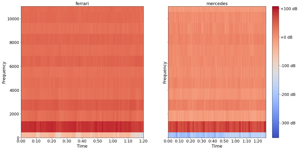
The plots above visualize the extracted MFCCs from the both sound-pieces. These extracted sound-pieces are now ready to be fed into a neural network. Before doing that though, we have to bulk-process all tracks instead of only these two. The following section elaborates on the implementation of this process.
Data Processing in bulk
When completing the final processing of all sound pieces to be fed into the neural network, it is important to notice that we do not have to go through all steps outlined above. Since the input features for our Deep Learning model is going to be a list of MFCCs, we can directly jump to this step. In addition to the necessary packages from before, we have to import several other packages for the following steps.
# Bulk processing packages
from pydub import AudioSegment
from pydub.utils import make_chunks
import math
import re
from tqdm import tqdm
import json
import copy
Before being able to process every race-track we have in our data, we should step back and ask ourselves a quite fundamental question in the realm of Neural Networks. Do we have enough data? Currently we have 19 sound-pieces, ten tracks with a mercedes engine and nine tracks with a ferrari engine. It is pretty clear to say that 19 observations are not going to be sufficient for training purposes.
There is luckily one work-around. Namely, it is possible to chop up every audio-track into one-second long snippets of sounds. The implications of that are tremendous. An audio-piece which has a length of around e.g. 80 seconds would then result into 80 pieces. Doing that for all tracks in our dataset, results in around 1000 audio snippets for Ferrari as well as for Mercedes. The following code shows how we split the longer audio-pieces into one-second-snippets.
raw_files = {
    "ferrari": r"{}/ferrari".format(raw_path),
    "mercedes": r"{}/mercedes".format(raw_path)
}
for team in ["ferrari", "mercedes", "montage"]:
    wav_files = os.listdir("{}/{}".format(raw_path, team))
    for file in wav_files:
        if not file.startswith("."):
            file_name = "{}/{}/{}".format(raw_path, team, file)
            myaudio = AudioSegment.from_file(file_name, "wav")
            chunk_length_ms = 1000
            chunks = make_chunks(myaudio, chunk_length_ms)
            for i, chunk in enumerate(chunks):
                padding = 3 - len(str(i))
                number = padding*"0" + str(i)
                chunk_name = "{}_{}".format(re.split(".wav", file)[0], number)
                chunk.export("{}/{}/{}.wav".format(data_path, team,
                                                    chunk_name), format="wav")
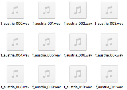
The resulting files of this code can be seen below. Here we can see the first twelve one-second-snippets of a Ferrari sound. From the name we can also infer where the sound was recorded: on the austrian race-track.
Next up is now the mass-extraction of the MFCCs for each of the different one-second-snippets. In order to avoid data leakage, we put aside two audio-pieces for both engines to have a clean test-dataset for later performance assessment.
Furthermore, for visual purposes we build a montage video which compromises several different snippets in order to better present our model performance. The following code shows the bulk processing for all three audio segments.
data = {
     "train": {"mfcc": [], "labels": [], "category": []},
     "test": {"mfcc": [], "labels": [], "category": []},
     "montage": {"mfcc": []}
}
test_tracks = ["f_austria", "m_australia"]
SAMPLE_RATE = 22050
n_mfcc = 13
n_fft = 2048
hop_length = 512
expected_num_mfcc_vectors = math.ceil(SAMPLE_RATE / hop_length)
for i, (dirpath, dirnames, filenames) in enumerate(os.walk(data_path)):
# ensure that we are not at the root level
    if dirpath is not data_path:
# save the team information
        dirpath_components = dirpath.split("/")
        label = dirpath_components[-1]
# looping over the wav files
        for f in tqdm(filenames):
            if not f.startswith("."):
                file_path = os.path.join(dirpath, f)
                signal, sr = librosa.load(file_path, sr=SAMPLE_RATE)
# extract the mfcc from the sound snippet
                mfcc = librosa.feature.mfcc(signal, sr=sr,
                                            n_fft=n_fft,
                                            n_mfcc=n_mfcc,
                                            hop_length=hop_length)
                mfcc = mfcc.T.tolist()
                # to ensure that all snippets have the same length
                if len(mfcc) == expected_num_mfcc_vectors:
if any([track in f for track in test_tracks]):
                        data["test"]["mfcc"].append(mfcc)
                        data["test"]["labels"].append(i-1)
                        data["test"]["category"].append(label)
                    elif ("montage" in f):
                        print(f)
                        data["montage"]["mfcc"].append(mfcc)
                    else:
                        data["train"]["mfcc"].append(mfcc)
                        data["train"]["labels"].append(i-1)
                        data["train"]["category"].append(label)
# saving json with the results
with open("{}/processed_data.json".format(data_path), "w") as fp:
    json.dump(data, fp, indent=4)
Lets take a look on the processed data. Here we can see from left to right the captured MFCCs, the label which indicates whether it is a Ferrari or a Mercedes, and the category which leaves no doubt what is meant with a label of zero.
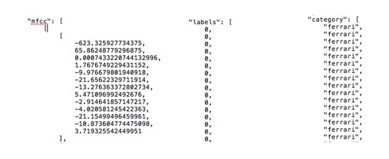
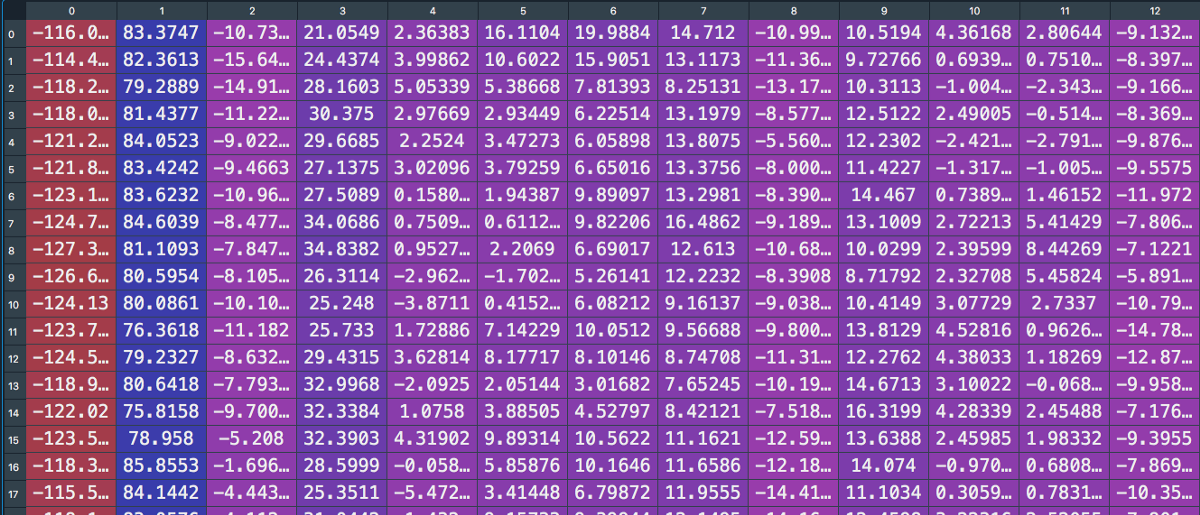
The MFCC values we see on the left side on the picture above are extracted from one Fourier Transform. As mentioned before, we use a frame size of 2048 to conduct the FFT, afterwards we shift 512 samples to the right and conduct the next FFT. Given that we have 22050 samples per second, we end up with 44 Fourier Transforms, and 44 vectors containing 13 extracted coefficients each. The image below shows an excerpt of the resulting matrix.
Neural Network
Finally it is time now to build our Neural Network. We start by loading in the data we saved earlier, and split test and training data using sklearn train_test_split command. Here we assign 20% to the test data before turning to the model architecture.
As can be seen from the image above, every one-second audio snippet consists of a matrix. Since we cannot really feed in a matrix in its current form into a neural network we define our first layer as a flattening layer. This is not anything other than bringing the data into a 1-D format. Given that we have 13 coefficients and 44 extraction cycles, our input layer will have a length of 13 x 44 = 572
Afterwards, we define three hidden layers with 512, 256 and 64 neurons, respectively. We also specify a 30% dropout layer in order to prevent overfitting. Since the output is binary we specify 1 as the output dimensionality. When compiling the network we use the compiler Adam and a learning rate of 0.0001. Furthermore, given that we have a binary problem (an engine either belongs to Ferrari or Mercedes) we use binary_crossentropy as our loss function.
# Importing packages
from sklearn.model_selection import train_test_split
import tensorflow.keras as keras
from sklearn.metrics import accuracy_score
# load and convert data
with open("{}/processed_data.json".format(data_path), "r") as fp:
    data = json.load(fp)
inputs = np.array(data["train"]["mfcc"])
targets = np.array(data["train"]["labels"])
# turn data into train and testset
(inputs_train, inputs_test,
 target_train, target_test) = train_test_split(inputs, targets,
                                               test_size=0.2)
# build the network architecture
model = keras.Sequential([
    # input layer
    keras.layers.Flatten(input_shape=(inputs.shape[1],
                                      inputs.shape[2])),
# 1st hidden layer
    keras.layers.Dense(512, activation="relu"),
    keras.layers.Dropout(0.3),
# 2nd hidden layer
    keras.layers.Dense(256, activation="relu"),
    keras.layers.Dropout(0.3),
# 3rd hidden layer
    keras.layers.Dense(64, activation="relu"),
    keras.layers.Dropout(0.3),
# output layer
    keras.layers.Dense(1, activation="sigmoid")
])
# compiling the network
optimizer = keras.optimizers.Adam(learning_rate=0.000_1)
model.compile(optimizer=optimizer, loss="binary_crossentropy",
              metrics=["accuracy"])
model.summary()
# train the network
history = model.fit(inputs_train, target_train,
                    validation_data=(inputs_test, target_test),
                    epochs=100,
                    batch_size=32)
After storing our training history it is now time to look at our results over all epochs. The following code graphs the accuracy as well as the error over the epochs.
fig, axs = plt.subplots(nrows=1, ncols=2, figsize=(20, 10))
# create accuracy subplot
axs[0].plot(history.history["accuracy"], label="train_accuracy")
axs[0].plot(history.history["val_accuracy"], label="test_accuracy")
axs[0].set_ylabel("Accuracy", fontsize=18)
axs[0].legend(loc="lower right", prop={"size": 16})
axs[0].set_title("Accuracy evaluation", fontsize=20)
axs[0].tick_params(axis="both", labelsize=16)
# create error subplot
axs[1].plot(history.history["loss"], label="train error")
axs[1].plot(history.history["val_loss"], label="test error")
axs[1].set_ylabel("Error", fontsize=18)
axs[1].legend(loc="upper right", prop={"size": 16})
axs[1].set_title("Error evaluation", fontsize=20)
axs[1].tick_params(axis="both", labelsize=16)
fig.savefig("{}/accuracy_error.png".format(output_path),
            bbox_inches="tight")
plt.show()
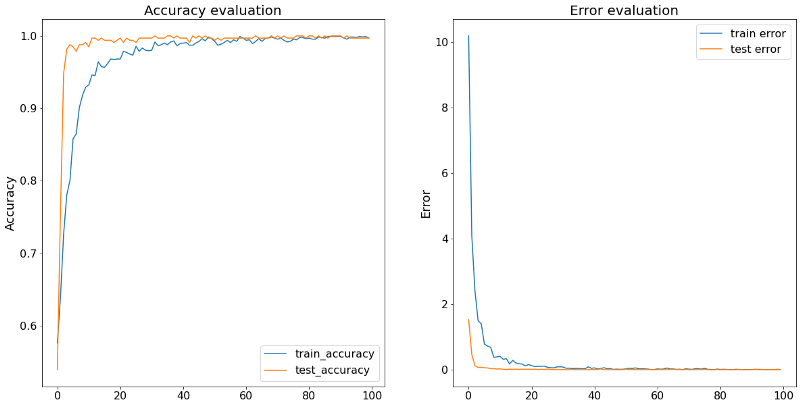
The result is pleasantly surprising. The model learns very quickly, and is nicely able to tell which sound belongs to which engine. To really test how well our models work, we have to see how they perform on data they haven’t seen before. We now apply the model on the two sound-pieces which we not used in the building of the neural network.
test_inputs = np.array(data["test"]["mfcc"])
test_targets = np.array(data["test"]["labels"])
predictions = model.predict_classes(test_inputs)
acc = accuracy_score(test_targets, predictions)
We assess the model’s accuracy with the code above. The accuracy is 98.79%, on the never-before-seen data, making it a very accurate predictor of engine sound.
Montage Video
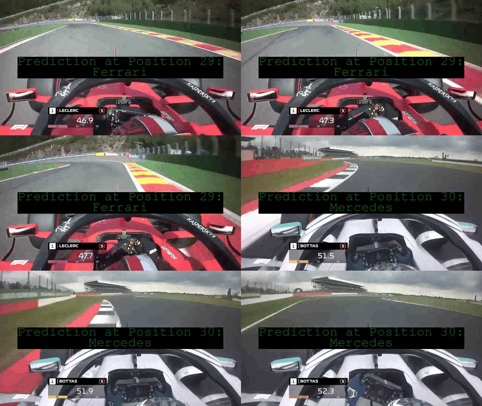
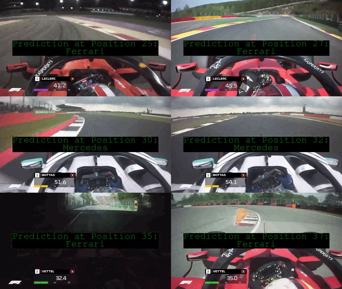
Lastly, as touched on earlier in this post, we build a small montage video which combines the sound-prediction with a visual to make the results come alive. For that we first predict the engine-brand using our priorly trained neural network. Afterwards, we store the results in a list, and replace the numeric label with a string.
montage_inputs = np.array(data["montage"]["mfcc"])
predictions = model.predict_classes(montage_inputs)
list_pred = [x.tolist()[0] for x in predictions]
engine_prediction = ["Mercedes" if x == 1 else "Ferrari" for x in list_pred]
Using the wonderful package moviepy we import the video and print the position of video (measured in seconds) and our prediction in the middle of the screen. Voila!
import moviepy.editor as mp
montage = mp.VideoFileClip("{}/video/montage.mp4".format(raw_path))
clip_list = []
for second, engine in tqdm(enumerate(engine_prediction)):
    engine_text = (mp.TextClip(
        "Prediction at Position {}:\n{}".format(second, engine),
        fontsize=70, color='green',
        bg_color="black")
        .set_duration(1)
        .set_start(0))
clip_list.append(engine_text)
final_clip = (mp.concatenate(clip_list, method="compose")
              .set_position(("center", "center")))
montage = mp.CompositeVideoClip([montage, final_clip])
montage.write_videofile(
    "{}/video/montage_with_text.mp4".format(raw_path),
    fps=24, codec="mpeg4")
Sources [1] https://www.youtube.com/watch?v=kmuKQ2JQK30&list=PLfoNZDHitwjUA9aqbPGKw1l4SIz2bACi_ [2] https://www.youtube.com/channel/UCZPFjMe1uRSirmSpznqvJfQ
